Information gain
Information gain is a splitting score that measures how much a split lowers entropy, so a decision tree can choose which feature to split on first.
Last updated: 04 Oct, 2026 · scikit-learn 1.9.1
Entropy and Gini impurity scores one node. A split creates several nodes at once, and the dataset offers several features to split on. Information gain turns the children's entropies into one number per candidate split, and the tree takes the largest.
Choosing which feature to split first
The board's example: a feature f1 splits the root, 9 Yes and 5 No, into two categories, C1 with 6 Yes and 2 No and C2 with 3 Yes and 3 No. Another feature f2 could split the same root into three categories. Should the tree start with f1 or f2? Compute the information gain of each and pick the larger.
H(S) is the entropy of the root. Sᵥ is the set of records that go to branch v, |Sᵥ| how many there are, and |S| the total. So the sum is the children's entropy, each weighted by its share of the records. First, the root:
Working out the gain of f1
Next the two children. C1 has 8 records, 6 Yes and 2 No; C2 has 6 records, 3 Yes and 3 No:
C1 holds 8 of the 14 records and C2 holds 6, so the weights are 8/14 and 6/14:
The video says 0.041 here and the board writes 0.049; the sum works out to 0.048 (0.049 comes from rounding 0.94 and 0.81 first).
Suppose the split on f2 gives Gain(S, f2) = 0.051, the board's example value. That is larger than f1's gain, so the tree starts with f2, even though the margin is small. The rule is the same at every node: compute the gain of every candidate split and take the highest.
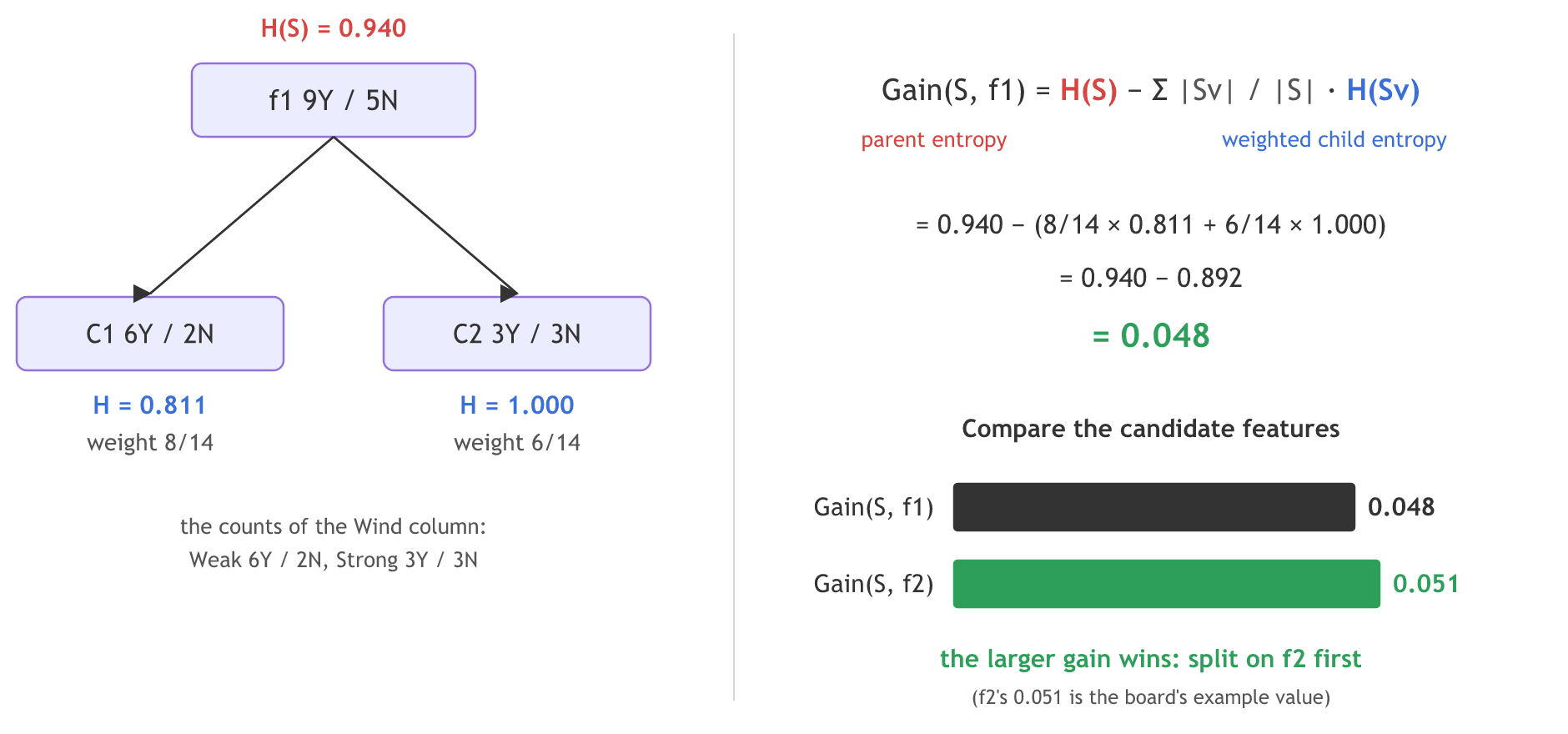
The counts on the board are those of the Wind column of play tennis: Weak days are 6 Yes and 2 No, Strong days 3 Yes and 3 No. The code below computes the gain of all four play-tennis features.
Splitting a numeric feature with thresholds
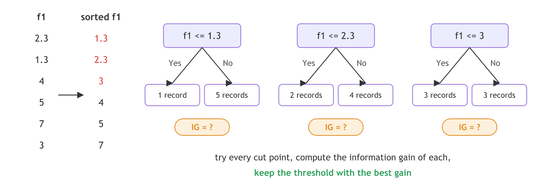
A numeric feature has no categories to branch on. The board's f1 has the values 2.3, 1.3, 4, 5, 7 and 3. The tree first sorts them: 1.3, 2.3, 3, 4, 5, 7.
Then it tries each value as a threshold. f1 ≤ 1.3 sends 1 record to the Yes branch and 5 to the No branch; compute the information gain. f1 ≤ 2.3 sends 2 and 4; compute the gain again. f1 ≤ 3 sends 3 and 3, and so on through the list. The threshold with the best information gain becomes the split. The sorted list ends at 7, as on the board; the clip reads the last value as 6.
The clip's column has no output. Give it one and the search becomes concrete. Seven records of f1, already sorted, 2.3, 3.6, 4, 5.2, 6.7, 8.9 and 10.5, have the outputs Yes, Yes, No, No, Yes, No, Yes: 4 Yes and 3 No, an entropy of 0.985. The cut f1 ≤ 2.3 sends 1 Yes to the left and leaves 3 Yes, 3 No on the right. The cut f1 ≤ 3.6 sends 2 Yes left and leaves 2 Yes, 3 No. Both left branches are pure, but the second cut also cleans up the right side more, so its information gain is higher: 0.292 against 0.128.
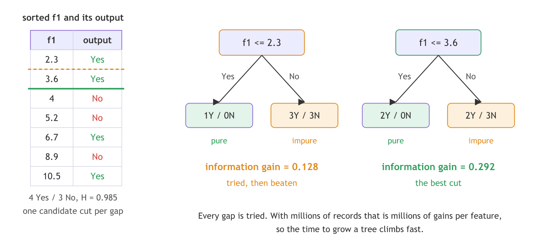
This search has a price. Every gap between two sorted values is a candidate cut, so a feature with millions of different values means millions of information gains at a single node. That is why growing a tree on large numeric data takes time.
Computing information gain in Python
The code needs the play-tennis table and the entropy function again, the same code as in Decision tree classifier and Entropy and Gini impurity.
Typing the play-tennis table
import pandas as pd

# The 14 days of the play-tennis table, one string per column
outlook = "Sunny Sunny Overcast Rain Rain Rain Overcast Sunny Sunny Rain Sunny Overcast Overcast Rain".split()
temperature = "Hot Hot Hot Mild Cool Cool Cool Mild Cool Mild Mild Mild Hot Mild".split()
humidity = "High High High High Normal Normal Normal High Normal Normal Normal High Normal High".split()
wind = "Weak Strong Weak Weak Weak Strong Strong Weak Weak Weak Strong Strong Weak Strong".split()
play = "No No Yes Yes Yes No Yes No Yes Yes Yes Yes Yes No".split()

df = pd.DataFrame({"Outlook": outlook, "Temperature": temperature,
                   "Humidity": humidity, "Wind": wind, "PlayTennis": play})
An entropy function
import numpy as np

def entropy(counts):
    p = np.array(counts) / sum(counts)
    p = p[p > 0]                      # 0 * log2(0) counts as 0
    return float((p * np.log2(1 / p)).sum())   # same as -sum(p * log2(p))
An information gain function
def information_gain(parent, children):
    # parent = [yes, no]; children = one [yes, no] list per branch
    n = sum(parent)
    weighted = sum(sum(c) / n * entropy(c) for c in children)
return entropy(parent) - weightedprint("Gain(S, f1) =", round(information_gain([9, 5], [[6, 2], [3, 3]]), 3))
for feature in ["Outlook", "Temperature", "Humidity", "Wind"]:
counts = pd.crosstab(df[feature], df["PlayTennis"])[["Yes", "No"]]
print(f"{feature:12}", counts.values.tolist(), round(information_gain([9, 5], counts.values.tolist()), 3))Gain(S, f1) = 0.048 Outlook [[4, 0], [3, 2], [2, 3]] 0.247 Temperature [[3, 1], [2, 2], [4, 2]] 0.029 Humidity [[3, 4], [6, 1]] 0.152 Wind [[3, 3], [6, 2]] 0.048
Finding the best threshold for f1
A sorted numeric column with its output
# A numeric feature f1 and its Yes/No output, 4 Yes and 3 No
f1 = [2.3, 3.6, 4, 5.2, 6.7, 8.9, 10.5]
label = ["Yes", "Yes", "No", "No", "Yes", "No", "Yes"]
pairs = sorted(zip(f1, label)) # sort by the feature valuefrom sklearn.tree import DecisionTreeClassifier
values = [v for v, _ in pairs]
labels = [lab for _, lab in pairs]
parent = [labels.count("Yes"), labels.count("No")]
for i, cut in enumerate(values[:-1]):
left, right = labels[: i + 1], labels[i + 1:]
children = [[left.count("Yes"), left.count("No")], [right.count("Yes"), right.count("No")]]
print(f"f1 <= {cut}: {len(left)} | {len(right)} records, gain {information_gain(parent, children):.3f}")
stump = DecisionTreeClassifier(criterion="entropy", max_depth=1).fit([[v] for v in f1], label)
print("scikit-learn threshold:", round(stump.tree_.threshold[0], 2))f1 <= 2.3: 1 | 6 records, gain 0.128 f1 <= 3.6: 2 | 5 records, gain 0.292 f1 <= 4: 3 | 4 records, gain 0.020 f1 <= 5.2: 4 | 3 records, gain 0.020 f1 <= 6.7: 5 | 2 records, gain 0.006 f1 <= 8.9: 6 | 1 records, gain 0.128 scikit-learn threshold: 3.8
What the gains show
- Gain(S, f1) = 0.048, the board's f1, computed without rounding.
- Outlook has the highest gain, 0.247, ahead of Humidity (0.152), Wind (0.048) and Temperature (0.029). That is why a tree on play tennis starts with Outlook.
- Wind's counts are [[3, 3], [6, 2]]: Strong and Weak, the board's C2 and C1.
- f1 ≤ 3.6 has the best gain, 0.292: 2 Yes on the left, a pure branch, and 2 Yes, 3 No on the right. f1 ≤ 2.3 and f1 ≤ 8.9 tie at 0.128, and the cuts in the middle gain almost nothing.
- scikit-learn puts the threshold at 3.8, halfway between 3.6 and 4. Any cut between the two values sends the records the same way; scikit-learn takes the midpoint.
Categorical feature vs numeric feature
| Categorical feature (Outlook) | Numeric feature (f1) | |
|---|---|---|
| Candidate splits | One, by category | One per gap between sorted values |
| Branches | One per category in the video's tree | Two: ≤ threshold and > threshold |
| What gets compared | The gain of each feature | The gain of each threshold, then the best one against other features |
| Example | Outlook: Sunny, Overcast, Rain | f1 ≤ 2.3, ≤ 3.6, ≤ 4, ... |
Where you use information gain
- Growing trees:
criterion="entropy"makes scikit-learn pick splits by information gain. - Ranking features:
mutual_info_classifinsklearn.feature_selectionscores features by the same idea, the information a feature gives about the class. - Explaining a model: the first split of a tree is the single most informative question in the data.
Related
- Previous: Entropy and Gini impurity
- Next: Decision tree regression and pruning
- Reference: scikit-learn user guide, decision tree mathematical formulation
- Add a Day column,
df["Day"] = [f"D{i}" for i in range(1, 15)], and compute its gain. Is it 0.940? - Change the output of the record 4 from No to Yes. Which threshold wins now, and where does scikit-learn put it?
- Add the
ginifunction from Entropy and Gini impurity (1 - (p ** 2).sum()on the class shares), swapentropyforginiinsideinformation_gainand rank the play-tennis features again. Does Outlook still come first?
Slow is fine. Stopping is the only problem.