Simple linear regression
Simple linear regression is a supervised learning algorithm that fits a straight line through data with one input feature to predict a continuous output.
Last updated: 05 Oct, 2026 · scikit-learn 1.9.1
It is the first algorithm in the video and the base for the rest of this part: the cost function, gradient descent and R² all start from this one line.
Fitting a best fit line
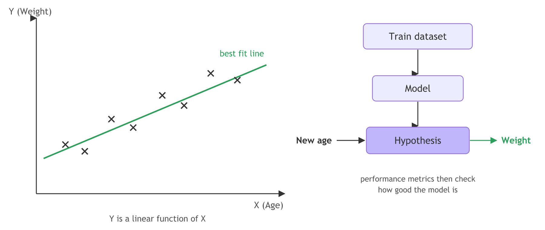
Take two features: X is age and Y is weight. Linear regression trains a model on this training dataset. The model is a hypothesis: it takes a new age and gives a weight. Performance metrics then check how well it does. In short, linear regression finds the best fit line through the points, and Y becomes a linear function of X. Why a straight line and not a curve comes up with the other algorithms later.
Writing the line three ways
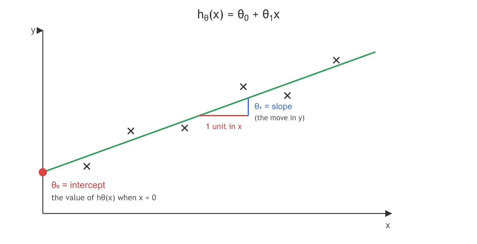
The same straight line has several notations: y = mx + c, y = β₀ + β₁x, and hθ(x) = θ₀ + θ₁x. The video uses the last one, from Andrew Ng's course, and so does this course.
| Notation | Intercept | Slope |
|---|---|---|
| y = mx + c | c | m |
| y = β₀ + β₁x | β₀ | β₁ |
| hθ(x) = θ₀ + θ₁x | θ₀ | θ₁ |
Reading the intercept and the slope
- θ₀ is the intercept. When x = 0, hθ(x) = θ₀: it is the point where the line meets the y axis.
- θ₁ is the slope, also called the coefficient. Move one unit along the x axis; the movement in y is the slope.
- x(i) is the i-th data point.
- ŷ (y hat) is the predicted point hθ(x) on the line, and y − ŷ is the error for that point: the distance the Cost function lesson adds up.
Fitting the age and weight data
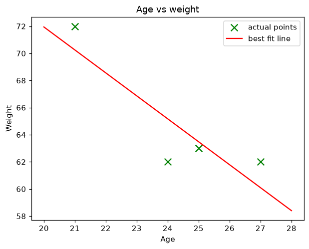
The video draws the line on the board. Here scikit-learn fits it to the video's own table: 24 and 62, 25 and 63, 21 and 72, 27 and 62.
The data as arrays
import numpy as np

# the board's table: age is the input, weight the output
age = np.array([[24], [25], [21], [27]])   # 2D: one row per person, one column per feature
weight = np.array([62, 63, 72, 62])
Passing a 1D array by mistake
scikit-learn wants X as a table, rows by features, even when there is one feature. A flat list of ages fails:
import numpy as np
from sklearn.linear_model import LinearRegression

ages_flat = np.array([24, 25, 21, 27])          # 1D: no feature column
LinearRegression().fit(ages_flat, [62, 63, 72, 62])Traceback (most recent call last):
File "main.py", line 5, in <module>
LinearRegression().fit(ages_flat, [62, 63, 72, 62])
ValueError: Expected 2D array, got 1D array instead:
array=[24 25 21 27].
Reshape your data either using array.reshape(-1, 1) if your data has a single feature or array.reshape(1, -1) if it contains a single sample.The fix is the double brackets in age above, or ages_flat.reshape(-1, 1).
Training LinearRegression
from sklearn.linear_model import LinearRegression

model = LinearRegression()   # fit_intercept=True by default, so it learns θ0
model.fit(age, weight)       # finds θ0 and θ1
Reading θ0 and θ1
theta0 = model.intercept_   # θ0
theta1 = model.coef_[0]     # θ1: coef_ holds one slope per feature
Predicting a weight from the line
import matplotlib.pyplot as plt

theta0, theta1 = model.intercept_, model.coef_[0]
print("θ0 (intercept):", round(theta0, 2))
print("θ1 (slope):    ", round(theta1, 2))
print("hθ(26) from predict:", round(model.predict([[26]])[0], 2))
print("hθ(26) by hand:     ", round(theta0 + theta1 * 26, 2))

line_x = np.array([[20], [28]])
plt.scatter(age, weight, color="green", marker="x", s=80, label="actual points")
plt.plot(line_x, model.predict(line_x), color="red", label="best fit line")
plt.title("Age vs weight")
plt.xlabel("Age")
plt.ylabel("Weight")
plt.legend()
plt.show()θ0 (intercept): 105.81 θ1 (slope): -1.69 hθ(26) from predict: 61.79 hθ(26) by hand: 61.79
What the slope and intercept mean
- θ₁ ≈ −1.69. Each extra year of age lowers the predicted weight by 1.69. The slope is negative because the 21-year-old weighs 72 while the others weigh 62 or 63; four rows are too few to show a real trend.
- θ₀ ≈ 105.81. The predicted weight at age 0. Age 0 is far outside the data, so the number has no meaning of its own; it fixes where the line sits.
- hθ(26) = 61.79 both ways.
predictcomputes θ₀ + θ₁ × 26, the hypothesis written out.
Fitting the notes' height and weight data
Four rows show the idea; the notes and the practical notebook use a bigger table. The notes predict a person's height from their weight: 74 kg is 170 cm, 80 kg is 180 cm, 75 kg is 175.5 cm. The notebook's height-weight.csv has 23 such people. It splits them, standardises the weights with the training rows (as in Train and test split) and fits the line.
Loading, splitting and scaling the table
import pandas as pd
from sklearn.model_selection import train_test_split
from sklearn.preprocessing import StandardScaler

url = ("https://raw.githubusercontent.com/krishnaik06/The-Grand-Complete-Data-Science-Materials/"
       "main/Machine%20Learning/2-Complete%20Linear%20Regression/Practicals/height-weight.csv")
df = pd.read_csv(url)
X_train, X_test, y_train, y_test = train_test_split(
    df[["Weight"]], df["Height"], test_size=0.25, random_state=42)
scaler = StandardScaler()
X_train = scaler.fit_transform(X_train)   # standardise with the train rows only
X_test = scaler.transform(X_test)
Training the height model
from sklearn.linear_model import LinearRegression

regression = LinearRegression()
regression.fit(X_train, y_train)   # finds the intercept and the slope
Predicting a height from a weight
import matplotlib.pyplot as plt

print("coefficient (slope):", regression.coef_.round(4))
print("intercept:", round(regression.intercept_, 4))
new_weight = scaler.transform(pd.DataFrame({"Weight": [72]}))   # scale it the same way
print("predicted height for 72 kg:", regression.predict(new_weight).round(2))

plt.scatter(X_train, y_train, color="green", label="training points")
plt.plot(X_train, regression.predict(X_train), color="red", label="best fit line")
plt.title("Weight vs height")
plt.xlabel("Weight (standardised)")
plt.ylabel("Height (cm)")
plt.legend()
plt.show()coefficient (slope): [17.2982] intercept: 156.4706 predicted height for 72 kg: [155.98]
What the height model learned
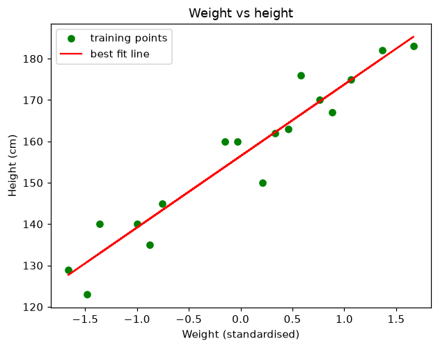
- The slope is 17.2982 and the intercept 156.4706, the same two numbers the notebook prints. So the line is height = 156.47 + 17.30 × (standardised weight).
- The slope is per standard deviation of weight, because the weights were standardised: one standard deviation heavier predicts 17.3 cm taller.
- The intercept is the average height of the 17 training people. A standardised weight of 0 is the average training weight, and the best fit line always passes through the average point.
- 72 kg predicts 155.98 cm, again the notebook's own answer. A new weight is scaled with the same
scalerbefore it goes into the model.
Simple vs multiple linear regression
| Simple linear regression | Multiple linear regression | |
|---|---|---|
| Inputs | One feature x | Several features x₁ … xₙ |
| Hypothesis | hθ(x) = θ₀ + θ₁x | hθ(x) = θ₀ + θ₁x₁ + … + θₙxₙ |
| Shape of the fit | A line | A plane, or a hyperplane |
coef_ | One value | One value per feature |
| Example | Age to weight | California housing to price, in Multiple linear regression |
Where you use simple linear regression
- A first model for any continuous target with one strong input, such as advertising spend and sales.
- Reading a trend: the slope says how much the output moves per unit of input.
- A baseline: a more complex model has to beat this line to be worth its cost.
model.predict([[60]]) returns 4.21, a weight no adult has, because the line keeps going down.Related
- Previous: Train and test split
- Next: Cost function
- Reference: LinearRegression
- Add a fifth person, age 30 and weight 75, to both arrays and refit: the slope turns positive.
- Fit the height model without the scaler (drop the three scaler lines): the slope becomes 1.048 cm per kg and the intercept 80.53, while the predictions stay the same.
- Fit with
LinearRegression(fit_intercept=False)on the age table: θ₀ becomes 0 and the line passes through the origin, the simplification the Cost function lesson uses.
Little by little, you're building something great.