DBSCAN
DBSCAN (density-based spatial clustering of applications with noise) is a clustering algorithm that grows clusters out of dense regions and leaves isolated points out as noise.
Last updated: 05 Oct, 2026 · scikit-learn 1.9.1
K-means clustering puts every point in some cluster, outliers included, and the Silhouette score cannot tell it that a point should belong nowhere. DBSCAN can leave an outlier out. It also finds clusters of any shape, and it does not need K.
Core points and the eps circle
The video lists the terms first: min points, core points, border points and noise points. Then it shows why they matter. With two groups and one point far from both, K-means still assigns that outlier to one of the groups. DBSCAN can call it a noise point and leave it out.
Two hyperparameters drive DBSCAN. Epsilon (ε) is the radius of a circle drawn around a point. MinPts is how many points that circle must hold. With MinPts = 4, a point whose ε circle holds at least 4 points is a core point, the red point on the board.
Border points, noise points and growing a cluster
The video first says a border point has at least one point inside its circle, then corrects it: at least one core point. A border point has fewer than MinPts points within ε, but lies within ε of a core point, so it joins that core point's cluster.
A noise point has no core point within ε. It is never put in a group; it is treated as an outlier. One sentence in the clip calls the noise point a cluster: it belongs to no cluster.
Core points within ε of each other are linked, so a chain of overlapping circles becomes one cluster, and its border points join it. The video's last picture compares a traditional method such as K-means, which puts the points in large blob-shaped groups, with DBSCAN, which gives each dense shape its own cluster and leaves the scattered points as noise.
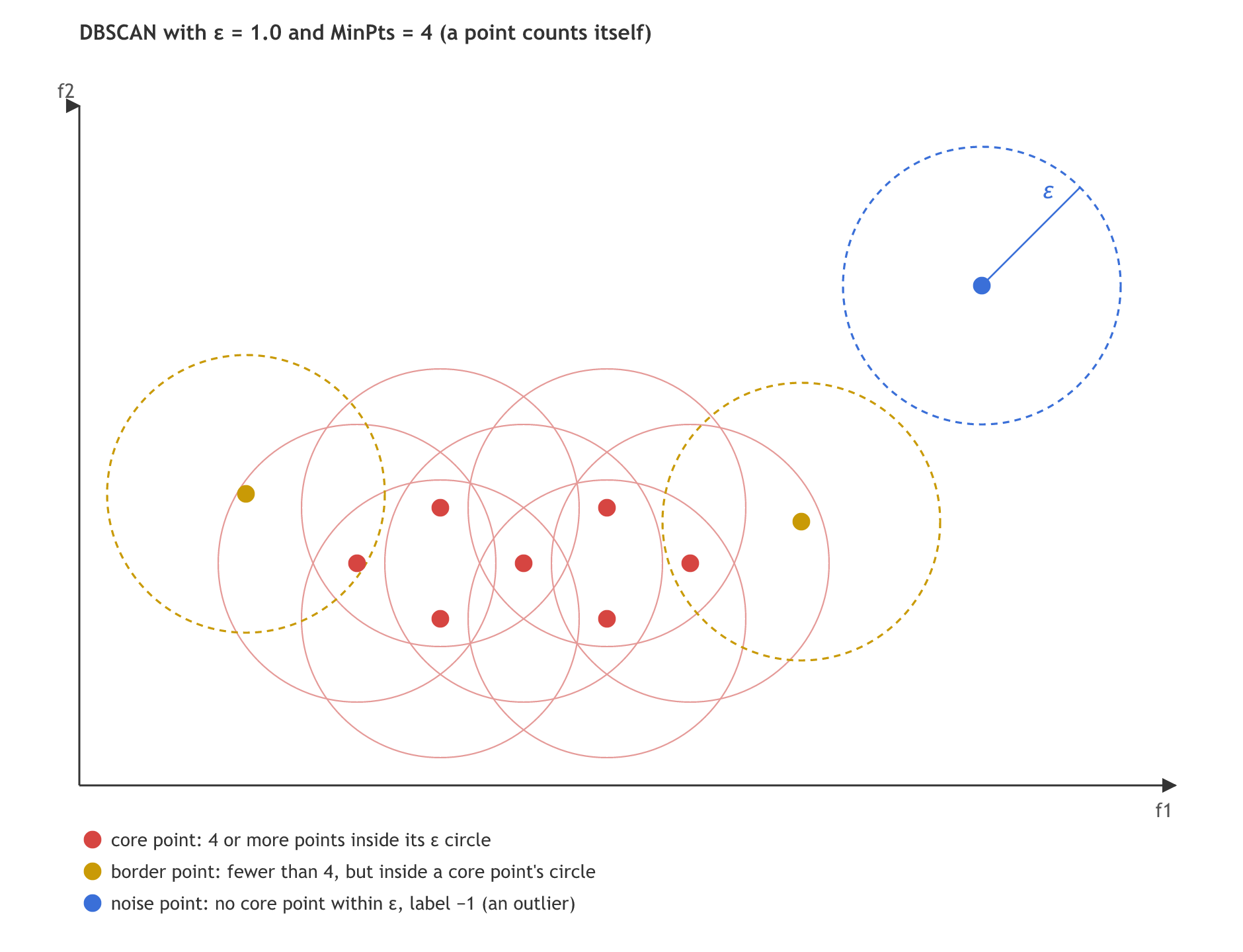
scikit-learn's min_samples counts the point itself, so min_samples=4 means the point plus three neighbours. The board notes take their definition from Wikipedia, which counts the point itself too: "at least 4 points (including the point itself)". The circle on the board holds four other points plus its centre, which is a core point under either reading.
Labelling core, border and noise points in scikit-learn
Fitting DBSCAN with eps and min_samples
from sklearn.cluster import DBSCAN

db = DBSCAN(eps=1.0, min_samples=4)   # ε radius and MinPts (the point counts itself)
db.fit(X)
print(db.labels_)                      # cluster number per point, -1 = noise
print(db.core_sample_indices_)         # positions of the core points
Telling border points from core points
labels_ gives the cluster but not the kind of point. core_sample_indices_ lists the core points, label -1 marks noise, and every other point is a border point.
import numpy as np

core = np.zeros(len(X), dtype=bool)
core[db.core_sample_indices_] = True
noise = db.labels_ == -1
border = ~core & ~noise        # in a cluster, but not a core point
Core, border and noise on ten points
import numpy as np
from sklearn.cluster import DBSCAN

X = np.array([[0, 0], [0.6, 0.4], [0.6, -0.4], [1.2, 0], [1.8, 0.4], [1.8, -0.4],
              [2.4, 0], [3.2, 0.3], [-0.8, 0.5], [4.5, 2.0]])

db = DBSCAN(eps=1.0, min_samples=4).fit(X)
core = np.zeros(len(X), dtype=bool)
core[db.core_sample_indices_] = True
noise = db.labels_ == -1
border = ~core & ~noise

print("labels_:", db.labels_)
for point, c, b in zip(X.tolist(), core, border):
    kind = "core" if c else ("border" if b else "noise")
print(f"{str(point):12} {kind}")labels_: [ 0 0 0 0 0 0 0 0 0 -1] [0.0, 0.0] core [0.6, 0.4] core [0.6, -0.4] core [1.2, 0.0] core [1.8, 0.4] core [1.8, -0.4] core [2.4, 0.0] core [3.2, 0.3] border [-0.8, 0.5] border [4.5, 2.0] noise
Reading labels_ == -1 as noise
- Seven core points, from [0, 0] to [2.4, 0], form one chain, cluster 0.
- [3.2, 0.3] and [-0.8, 0.5] are border points: their circles hold only themselves and one core point, so they join cluster 0 without being core points.
- [4.5, 2.0] gets label -1: no core point is within 1.0 of it, so it is noise, an outlier that belongs to no cluster.
Clustering two moons and an outlier
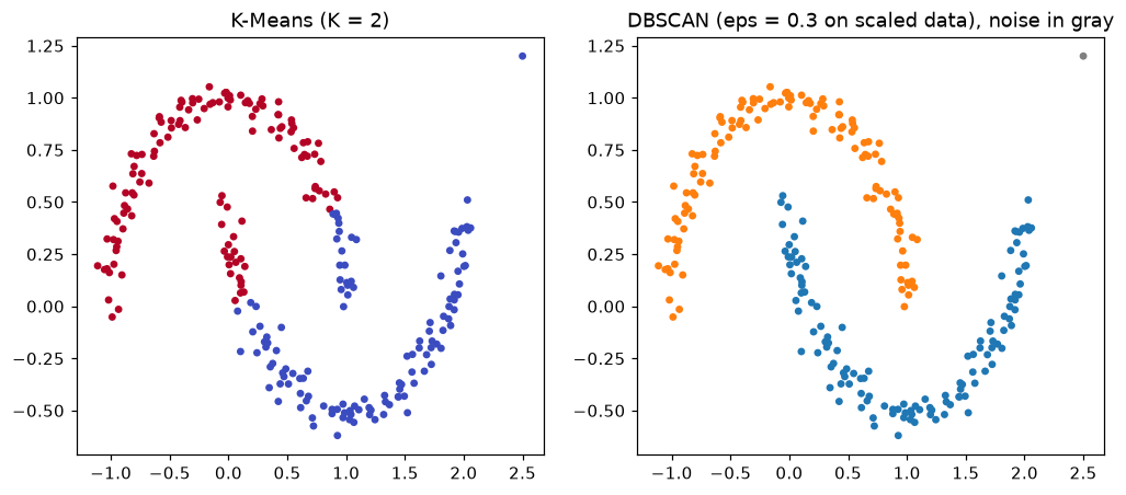
The DBSCAN notebook in the course materials makes 250 points in two interleaved half circles with make_moons(n_samples=250, noise=0.05), scales them with StandardScaler and fits DBSCAN(eps=0.3), leaving min_samples at its default. The run below does the same with random_state=0 and min_samples=5 written out, adds one outlier far from both moons, and fits K-means next to it. adjusted_rand_score compares a clustering with the true moons: 1.0 is a perfect match.
import numpy as np
import matplotlib.pyplot as plt
from sklearn.datasets import make_moons
from sklearn.preprocessing import StandardScaler
from sklearn.cluster import KMeans, DBSCAN
from sklearn.metrics import adjusted_rand_score

X, y = make_moons(n_samples=250, noise=0.05, random_state=0)
X = np.vstack([X, [[2.5, 1.2]]])                  # one outlier far from both moons
X_scaled = StandardScaler().fit_transform(X)      # eps is a distance, so scale first

km = KMeans(n_clusters=2, random_state=0).fit_predict(X_scaled)
db = DBSCAN(eps=0.3, min_samples=5).fit_predict(X_scaled)

print("K-means labels:", sorted(set(km.tolist())), " outlier ->", km[-1])
print("DBSCAN labels :", sorted(set(db.tolist())), " outlier ->", db[-1])
# 1.0 = the moons found exactly, 0 = no better than chance (outlier left out)
print("match with the true moons, K-means:", round(adjusted_rand_score(y, km[:250]), 3))
print("match with the true moons, DBSCAN :", round(adjusted_rand_score(y, db[:250]), 3))

fig, (ax1, ax2) = plt.subplots(1, 2, figsize=(11, 4.5))
ax1.scatter(X[:, 0], X[:, 1], c=km, cmap="coolwarm", s=12)
ax1.set_title("K-Means (K = 2)")
colors = np.where(db == -1, "gray", np.where(db == 0, "tab:blue", "tab:orange"))
ax2.scatter(X[:, 0], X[:, 1], c=colors, s=12)
ax2.set_title("DBSCAN (eps = 0.3 on scaled data), noise in gray")
plt.show()K-means labels: [0, 1] outlier -> 0 DBSCAN labels : [-1, 0, 1] outlier -> -1 match with the true moons, K-means: 0.439 match with the true moons, DBSCAN : 1.0
What the moons run shows
- K-means has no noise label: the outlier at (2.5, 1.2) is put in cluster 0 like every other point.
- K-means cuts across the moons with a straight line, so its match with the true moons is only 0.439.
- DBSCAN finds both moons exactly (match 1.0) and gives the outlier label -1, as the notebook's two plots show: the DBSCAN labels and the true moons look the same.
DBSCAN vs K-means
| DBSCAN | K-means | |
|---|---|---|
| Number of clusters | found from the data | K given up front |
| Cluster shape | any shape a chain of dense points makes | round groups around centroids |
| Outliers | labelled -1 and left out | always put in a cluster |
| Hyperparameters | eps and min_samples | K (and the init) |
Where you use DBSCAN
- Location data: GPS points cluster into the places people visit, and stray readings drop out as noise.
- Outlier detection: the points labelled -1 are the unusual transactions or sensor readings.
- Odd-shaped groups: regions in maps or images that are not round blobs.
Related
- Previous: Silhouette score
- Next: Curse of dimensionality
- Reference: scikit-learn user guide: DBSCAN
- In the moons example, change eps=0.3 to eps=0.2 and then to eps=0.7, and read the DBSCAN labels and match each time.
- Raise min_samples=4 to min_samples=5 in the ten-point example and see how many core points are left.
- In the moons example, move the outlier from [2.5, 1.2] to [1.0, 0.0], a spot on the lower moon, and check that DBSCAN no longer labels it -1.
Slow is fine. Stopping is the only problem.