Naive Bayes worked example
The Naive Bayes worked example is a hand calculation that predicts whether a person plays tennis from the Outlook and Temperature of the day, using counts from a 14-day table.
Last updated: 04 Oct, 2026 · scikit-learn 1.9.1
Naive Bayes ended with a formula: multiply the prior P(class) by one P(feature | class) per feature, then normalise. Here every one of those numbers is counted from a real table, and the same prediction is then made with scikit-learn.
Reading the play-tennis dataset
The video copies in a classic table of 14 days. The input features are Outlook, Temperature, Humidity and Wind. The output, PlayTennis, is Yes or No, so this is binary classification. Over the 14 days there are 9 Yes and 5 No.
| Day | Outlook | Temperature | Humidity | Wind | PlayTennis |
|---|---|---|---|---|---|
| D1 | Sunny | Hot | High | Weak | No |
| D2 | Sunny | Hot | High | Strong | No |
| D3 | Overcast | Hot | High | Weak | Yes |
| D4 | Rain | Mild | High | Weak | Yes |
| D5 | Rain | Cool | Normal | Weak | Yes |
| D6 | Rain | Cool | Normal | Strong | No |
| D7 | Overcast | Cool | Normal | Strong | Yes |
| D8 | Sunny | Mild | High | Weak | No |
| D9 | Sunny | Cool | Normal | Weak | Yes |
| D10 | Rain | Mild | Normal | Weak | Yes |
| D11 | Sunny | Mild | Normal | Strong | Yes |
| D12 | Overcast | Mild | High | Strong | Yes |
| D13 | Overcast | Hot | Normal | Weak | Yes |
| D14 | Rain | Mild | High | Strong | No |
Building the Outlook frequency table
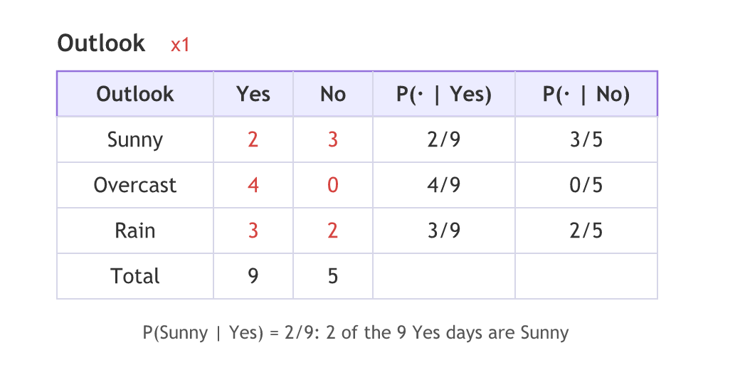
Outlook (x1) has three categories: Sunny, Overcast and Rain. For each one, count the Yes days and the No days. Sunny days: D1, D2 and D8 are No, D9 and D11 are Yes, so Sunny is 2 Yes and 3 No. Overcast is 4 Yes and 0 No. Rain is 3 Yes and 2 No. The columns add up to 9 Yes and 5 No.
Then turn counts into probabilities. Divide the Yes column by 9, the number of Yes days, and the No column by 5. The column the board heads P(Y) is P(Outlook | Yes): P(Sunny | Yes) = 2/9, P(Overcast | Yes) = 4/9, P(Rain | Yes) = 3/9. The No column gives 3/5, 0/5 and 2/5.
Building the Temperature table and the priors
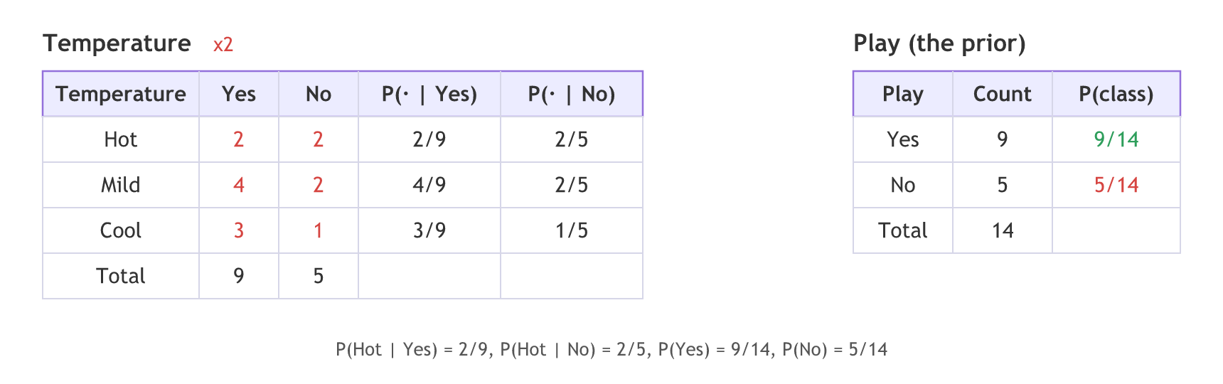
Temperature (x2) is counted the same way: Hot is 2 Yes and 2 No, Mild is 4 Yes and 2 No, Cool is 3 Yes and 1 No. Again the totals are 9 and 5, so P(Hot | Yes) = 2/9 and P(Hot | No) = 2/5.
The last table is the output itself. Out of 14 days, 9 are Yes and 5 are No, so the priors are P(Yes) = 9/14 and P(No) = 5/14.
The board labels the third row "Cold"; the dataset's value is Cool, which the counts here use.
Predicting a Sunny, Hot day
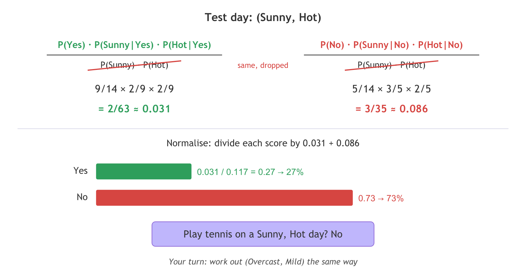
A new day arrives: Outlook is Sunny and Temperature is Hot. Write the Yes score and the No score, and drop the shared denominator P(Sunny) · P(Hot):
3/35 is 0.0857, which the board writes as 0.085. Normalising the two scores gives the answer:
On a Sunny, Hot day the person does not play tennis. The video leaves one more day as an assignment: (Overcast, Mild). It is the first Try-it item below.
Building the likelihood tables with pandas
The same tables come out of pandas in a few lines. pd.crosstab counts how often each pair of values appears, which is the frequency table from the board.
Typing the play-tennis table
import pandas as pd

# The 14 days of the play-tennis table, one string per column
outlook = "Sunny Sunny Overcast Rain Rain Rain Overcast Sunny Sunny Rain Sunny Overcast Overcast Rain".split()
temperature = "Hot Hot Hot Mild Cool Cool Cool Mild Cool Mild Mild Mild Hot Mild".split()
humidity = "High High High High Normal Normal Normal High Normal Normal Normal High Normal High".split()
wind = "Weak Strong Weak Weak Weak Strong Strong Weak Weak Weak Strong Strong Weak Strong".split()
play = "No No Yes Yes Yes No Yes No Yes Yes Yes Yes Yes No".split()

df = pd.DataFrame({"Outlook": outlook, "Temperature": temperature,
                   "Humidity": humidity, "Wind": wind, "PlayTennis": play})
Counting Yes and No per category
# Rows = categories of the feature, columns = No / Yes, plus a Total row
outlook_counts = pd.crosstab(df["Outlook"], df["PlayTennis"], margins=True, margins_name="Total")
temp_counts = pd.crosstab(df["Temperature"], df["PlayTennis"], margins=True, margins_name="Total")
Turning counts into P(category | class)
# P(category | class): divide each column by its class total (9 Yes, 5 No)
def likelihood(feature):
    counts = pd.crosstab(df[feature], df["PlayTennis"])
    return counts / counts.sum()

p_outlook = likelihood("Outlook")
p_temp = likelihood("Temperature")
prior = df["PlayTennis"].value_counts() / len(df) # P(Yes) = 9/14, P(No) = 5/14print(outlook_counts, "\n")
print(temp_counts, "\n")
print(p_outlook.round(3), "\n")
# The test day (Sunny, Hot): prior x P(Sunny | class) x P(Hot | class)
score = {c: float(prior[c] * p_outlook.loc["Sunny", c] * p_temp.loc["Hot", c]) for c in ["Yes", "No"]}
print({c: round(s, 4) for c, s in score.items()})
total = sum(score.values())
print({c: round(s / total, 2) for c, s in score.items()})PlayTennis No Yes Total
Outlook
Overcast 0 4 4
Rain 2 3 5
Sunny 3 2 5
Total 5 9 14
PlayTennis No Yes Total
Temperature
Cool 1 3 4
Hot 2 2 4
Mild 2 4 6
Total 5 9 14
PlayTennis No Yes
Outlook
Overcast 0.0 0.444
Rain 0.4 0.333
Sunny 0.6 0.222
{'Yes': 0.0317, 'No': 0.0857}
{'Yes': 0.27, 'No': 0.73}What the tables and scores show
- The Outlook counts match the board: Sunny 3 No and 2 Yes, Overcast 0 and 4, Rain 2 and 3, Total 5 and 9. pandas sorts the columns alphabetically, so No comes before Yes.
- The Temperature counts match too: Hot 2 and 2, Mild 2 No and 4 Yes, Cool 1 No and 3 Yes.
- P(Sunny | No) = 0.6 and P(Sunny | Yes) = 0.222: these are 3/5 and 2/9 from the board, as decimals.
- The scores 0.0317 and 0.0857 are 2/63 and 3/35. After normalising, No gets 0.73 and Yes 0.27, the board's answer.
Running CategoricalNB on the same data
scikit-learn's CategoricalNB is the Naive Bayes model for features made of categories. It counts the same tables during fit, with one difference: it adds a small number alpha to every count before dividing. This is called smoothing.
Encoding the categories as numbers
from sklearn.preprocessing import OrdinalEncoder

# CategoricalNB wants each category as an integer code: Overcast=0, Rain=1, Sunny=2, ...
X = df[["Outlook", "Temperature"]]
y = df["PlayTennis"]
encoder = OrdinalEncoder()
X_codes = encoder.fit_transform(X)
Fitting CategoricalNB and asking about Sunny, Hot
from sklearn.naive_bayes import CategoricalNB

# alpha is the smoothing count added to every category (1.0 by default)
model = CategoricalNB(alpha=1.0)
model.fit(X_codes, y)
test = encoder.transform(pd.DataFrame([["Sunny", "Hot"]], columns=X.columns))
print(model.classes_, model.predict_proba(test))for alpha in [1.0, 1e-10]:
model = CategoricalNB(alpha=alpha).fit(X_codes, y)
proba = model.predict_proba(test)[0]
print(f"alpha={alpha}: classes {model.classes_.tolist()} -> {proba.round(3)} -> {model.predict(test)[0]}")alpha=1.0: classes ['No', 'Yes'] -> [0.625 0.375] -> No alpha=1e-10: classes ['No', 'Yes'] -> [0.73 0.27] -> No
Why alpha changes the numbers
With the default alpha = 1.0 the model says 0.625 No and 0.375 Yes, not 0.73 and 0.27. With alpha close to 0 it gives exactly the hand result. Smoothing adds alpha to every count and alpha times the number of categories to every total:
- P(Sunny | Yes) becomes (2 + 1) / (9 + 1 × 3) = 3/12 = 0.25 instead of 2/9 = 0.222.
- P(Sunny | No) becomes (3 + 1) / (5 + 3) = 0.5 instead of 0.6. On only 5 No days, adding 1 to each count moves the numbers a lot, so the No side loses some of its lead.
- Both settings still answer No. Smoothing changes how sure the model is, not the winner here.
Hand count vs CategoricalNB
| Hand count (pandas) | CategoricalNB | |
|---|---|---|
| Likelihood | count / class total | (count + alpha) / (class total + alpha · k) |
| A category never seen with a class | Probability 0, wipes out the whole product | Small but not 0 |
| Sunny, Hot | No 0.73, Yes 0.27 | No 0.625, Yes 0.375 (alpha = 1) |
| Input | Category names | Integer codes from OrdinalEncoder |
Where you use Naive Bayes on categories
- Survey and form data: answers such as region, plan type or device, where every feature is a category.
- Quick weather or event tables: small datasets like this one, where counting is the whole model and you can check it by hand.
- Word counts: for text, the related
MultinomialNBuses the same counting and the same alpha smoothing on word counts.
encoder.transform.Related
- Previous: Naive Bayes
- Next: K nearest neighbours (KNN)
- Reference: CategoricalNB in the scikit-learn API reference
- Do the video's assignment: change the test day to ("Overcast", "Mild") in the pandas example. Work out 9/14 × 4/9 × 4/9 for Yes by hand first, then look at the No score and explain why it is 0.
- Run the same ("Overcast", "Mild") day through CategoricalNB with alpha=1.0. Is No still at 0?
- Add Humidity as a third feature: build
p_hum = likelihood("Humidity")and multiply in P(High | class) for a (Sunny, Hot, High) day.
This is what real progress feels like.