Machine learning workflow
A machine learning workflow is the fixed order of steps that takes a dataset to a model whose score you can trust: look at the data, split it once, put the preprocessing and the model in one pipeline, compare models with cross-validation on the training rows, tune the best one, and score it once on the test rows.
Last updated: 05 Oct, 2026 · scikit-learn 1.9.1
Every earlier lesson taught one algorithm. Here they all run on one dataset, in the order the video's practicals use them, so the result is a model and a test score you can defend. The same order also explains how a score can come out higher than the model deserves, and that is shown with real output.
Following the workflow from data to test score
The practicals in the video follow one order. In Logistic regression in scikit-learn it loads the breast cancer data, checks the class counts with value_counts(), splits the rows with train_test_split, tunes the model with GridSearchCV(scoring='f1', cv=5) and ends with confusion_matrix and classification_report on the test rows. The workflow below keeps that order and adds two things the later lessons taught: a Pipeline with StandardScaler, and a comparison of several models before tuning.
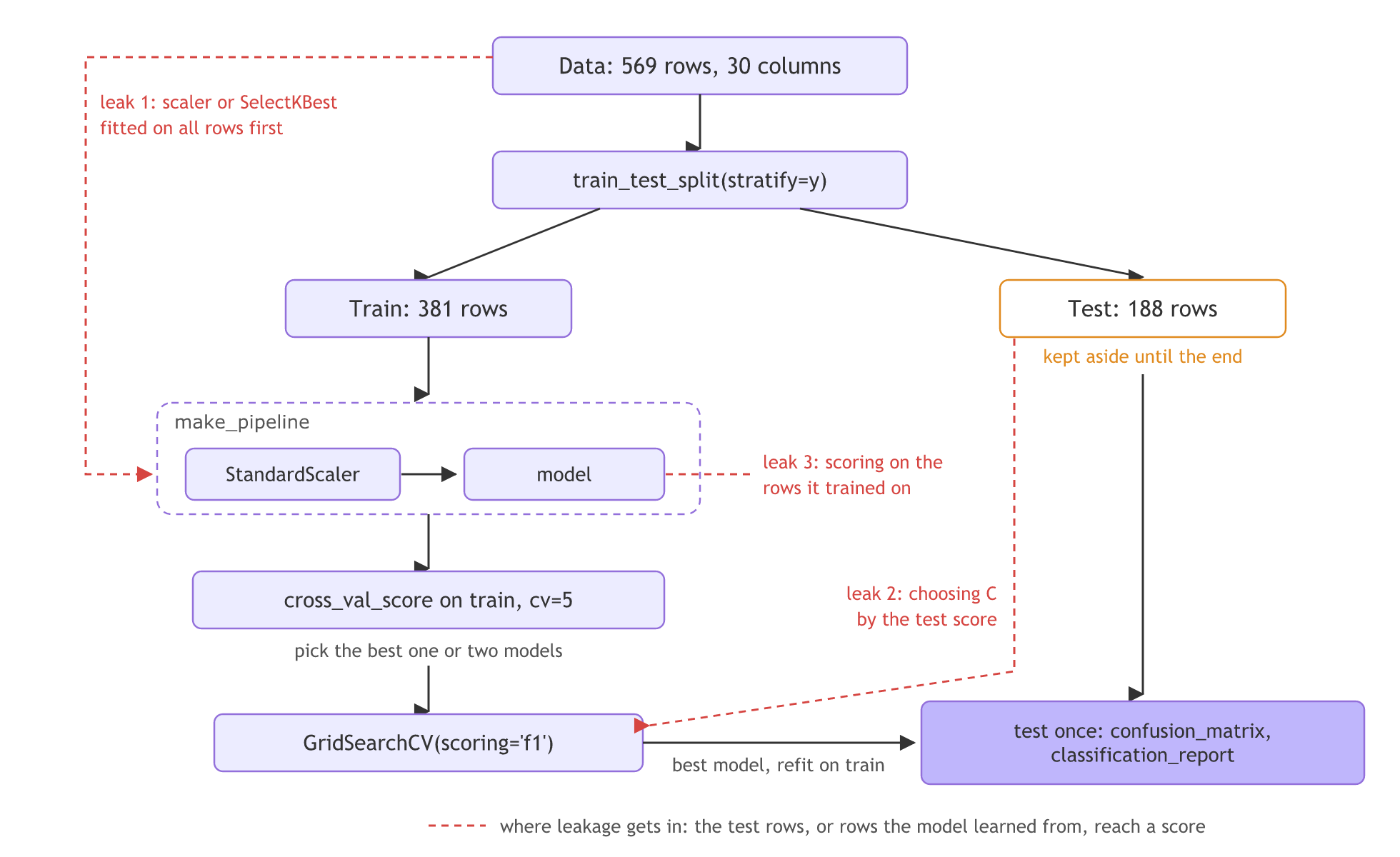
Every step below the train box uses the 381 training rows only. The 188 test rows wait on the right and are used once, at the end. The red dashed arrows are the three places where information from the test rows, or from the rows the model learned from, can reach a score. That is called data leakage, and each one is run later in this lesson.
Loading the breast cancer data
The dataset has 30 measurements of cell nuclei from 569 breast tumour samples. The target is 0 for malignant and 1 for benign. As in the video, the features go into a DataFrame X and the target into y, and value_counts() shows how many rows each class has.
import pandas as pd
from sklearn.datasets import load_breast_cancer

df = load_breast_cancer()
X = pd.DataFrame(df["data"], columns=df["feature_names"])
y = pd.Series(df["target"], name="Target")     # 0 = malignant, 1 = benign

print(X.shape)
print(X.iloc[:3, :4])
print(y.value_counts())(569, 30) mean radius mean texture mean perimeter mean area 0 17.99 10.38 122.8 1001.0 1 20.57 17.77 132.9 1326.0 2 19.69 21.25 130.0 1203.0 Target 1 357 0 212 Name: count, dtype: int64
There are 357 benign and 212 malignant rows, about 63% and 37%. The video calls this balanced: neither class is rare, so accuracy and f1 both mean something. With 30 columns on very different scales (mean area is in the hundreds, mean smoothness near 0.1), the distance-based models need scaling.
Splitting the rows once with stratify
The split is the same as the video's, test_size=0.33 and random_state=42, plus stratify=y. Stratifying keeps the 63/37 class mix in both parts, so the test rows look like the data the model will meet. The split happens once, before anything is fitted. Train and test split covers the arguments.
from sklearn.model_selection import train_test_split

X_train, X_test, y_train, y_test = train_test_split(
    X, y, test_size=0.33, random_state=42, stratify=y)

print("train:", X_train.shape, " test:", X_test.shape)
print("benign share, train:", round(y_train.mean(), 3), " test:", round(y_test.mean(), 3))train: (381, 30) test: (188, 30) benign share, train: 0.627 test: 0.628
381 rows train the models and 188 rows test the final one. Both parts keep the benign share at 0.627 and 0.628, the same as the full data.
Comparing seven classifiers with cross-validation
Each model from the course goes into the same pipeline: make_pipeline(StandardScaler(), model). A pipeline is one object, so cross_val_score refits the scaler on the four training folds every time and only transforms the fifth. The score is f1, as in the video's logistic practical, and it is computed on the training rows only. Cross-validation explains the five folds. XGBClassifier comes from the xgboost package; on macOS it also needs brew install libomp, as Installing scikit-learn explains.
Scaling inside the pipeline
pipe = make_pipeline(StandardScaler(), KNeighborsClassifier())
# fit: the scaler learns the mean and spread of the training folds, then KNN is fitted
# predict: the held-out fold is scaled with those numbers, never with its own
scores = cross_val_score(pipe, X_train, y_train, cv=5, scoring="f1")
Trees do not need scaling, because a split on one column does not depend on the other columns' units. Keeping them in the same pipeline does no harm and keeps the loop the same for every model.
Scoring every model on the training rows
from sklearn.model_selection import cross_val_score
from sklearn.pipeline import make_pipeline
from sklearn.preprocessing import StandardScaler
from sklearn.linear_model import LogisticRegression
from sklearn.neighbors import KNeighborsClassifier
from sklearn.naive_bayes import GaussianNB
from sklearn.tree import DecisionTreeClassifier
from sklearn.ensemble import RandomForestClassifier
from sklearn.svm import SVC
from xgboost import XGBClassifier

models = {
    "Logistic regression": LogisticRegression(),
    "KNN": KNeighborsClassifier(),
    "Naive Bayes": GaussianNB(),
    "Decision tree": DecisionTreeClassifier(random_state=42),
    "Random forest": RandomForestClassifier(random_state=42),
    "SVC": SVC(),
    "XGBoost": XGBClassifier(random_state=42),
}
for name, model in models.items():
    pipe = make_pipeline(StandardScaler(), model)   # the scaler is refit inside every fold
    scores = cross_val_score(pipe, X_train, y_train, cv=5, scoring="f1")
print(f"{name:20} f1 {scores.mean():.3f} +/- {scores.std():.3f}")Logistic regression f1 0.979 +/- 0.011 KNN f1 0.973 +/- 0.005 Naive Bayes f1 0.948 +/- 0.021 Decision tree f1 0.944 +/- 0.006 Random forest f1 0.967 +/- 0.008 SVC f1 0.973 +/- 0.014 XGBoost f1 0.969 +/- 0.007
What the cross-validation scores say
- Logistic regression leads with 0.979, then SVC and KNN at 0.973. On this data the classes are close to linearly separable, so a straight boundary is enough.
- The ensembles sit close behind: random forest 0.967 and XGBoost 0.969. They are strong models, but more flexibility does not help when a line already fits.
- A single decision tree is lowest at 0.944, with Naive Bayes at 0.948. An unpruned tree overfits its training folds, which the leakage section shows in numbers.
- The +/- is the spread over the five folds. Gaps of 0.006 between the top three are inside that spread, so the top two go on to tuning rather than only the top one.
Tuning logistic regression and SVC with GridSearchCV
Hyperparameter tuning with GridSearchCV tried every value in a grid with cross-validation. With a pipeline, a parameter name is the step name, two underscores, then the parameter: make_pipeline names each step after its class in lower case.
Naming a parameter inside a pipeline
pipe = make_pipeline(StandardScaler(), SVC())
print(pipe.steps[1][0])                   # 'svc'
grid = {"svc__C": [0.1, 1, 10, 100],      # C of the SVC step
        "svc__gamma": ["scale", 0.01, 0.001]}
The video's grid for logistic regression is [{'C':[1,5,10]},{'max_iter':[100,150]}], a list of two separate grids that never tries C and max_iter together. One dict per model, as below, tries every combination. Both searches use scoring='f1' and cv=5, like the video.
Searching the two grids
from sklearn.model_selection import GridSearchCV

logistic = GridSearchCV(make_pipeline(StandardScaler(), LogisticRegression()),
                        {"logisticregression__C": [0.01, 0.1, 1, 10, 100]},
                        scoring="f1", cv=5).fit(X_train, y_train)
svc = GridSearchCV(make_pipeline(StandardScaler(), SVC()),
                   {"svc__C": [0.1, 1, 10, 100], "svc__gamma": ["scale", 0.01, 0.001]},
                   scoring="f1", cv=5).fit(X_train, y_train)

for name, search in (("Logistic regression", logistic), ("SVC", svc)):
print(f"{name:20} best f1 {search.best_score_:.3f} {search.best_params_}")Logistic regression best f1 0.982 {'logisticregression__C': 0.1}
SVC best f1 0.980 {'svc__C': 1, 'svc__gamma': 0.01}What the two searches chose
- Logistic regression with C = 0.1 reaches 0.982, up from 0.979 with the default C = 1. A smaller C is a stronger penalty on the weights, the same idea as ridge regression's λ in reverse.
- SVC with C = 1 and gamma = 0.01 reaches 0.980, up from 0.973.
- Logistic regression is the pick, because its cross-validated f1 is higher. The choice is made before the test rows are touched.
Testing the chosen model once
best_estimator_ is the winning pipeline refitted on all 381 training rows. It predicts the 188 test rows once, and the video's two reports read the result. Confusion matrix and Precision, recall and F-beta explain each number.
from sklearn.metrics import confusion_matrix, classification_report

best = logistic.best_estimator_     # chosen by the cross-validated f1 on the train rows
y_pred = best.predict(X_test)       # the first and only look at the test rows
print(confusion_matrix(y_test, y_pred))
print(classification_report(y_test, y_pred, target_names=df["target_names"], digits=3))[[ 68 2]
[ 1 117]]
precision recall f1-score support
malignant 0.986 0.971 0.978 70
benign 0.983 0.992 0.987 118
accuracy 0.984 188
macro avg 0.984 0.981 0.983 188
weighted avg 0.984 0.984 0.984 188Reading the test report
- The confusion matrix has 3 errors in 188 rows. Rows are the true class and columns the prediction: 68 malignant found, 2 malignant called benign (false negatives for cancer), 1 benign called malignant, 117 benign right.
- Test f1 for benign is 0.987 and accuracy 0.984, close to the cross-validated 0.982. A test score near the CV score is the sign that the workflow did not leak.
- Malignant recall is 0.971. In the video's spam vs cancer example, a missed cancer costs more than a false alarm, so this is the number to push up next, for example by moving the decision threshold so that fewer tumours are called benign.
Leaking the test rows into the score
Each leak below makes a score look better than the model is. The code runs on the same data and prints the leaked number next to the honest one.
Scoring a deep tree on its own training rows
A decision tree with no depth limit keeps splitting until every leaf is pure. Scored on the rows it learned from, it has memorised the answers.
from sklearn.tree import DecisionTreeClassifier

tree = DecisionTreeClassifier(random_state=42).fit(X_train, y_train)   # no depth limit
print("depth of the tree:", tree.get_depth())
print(f"accuracy on the rows it trained on: {tree.score(X_train, y_train):.3f}")
print(f"accuracy on the test rows: {tree.score(X_test, y_test):.3f}")depth of the tree: 6 accuracy on the rows it trained on: 1.000 accuracy on the test rows: 0.904
Accuracy 1.000 on the training rows and 0.904 on the test rows. The 1.000 measures memory, not prediction. This is the overfitting from Overfitting and underfitting: low bias, high variance. Cross-validation would have reported the honest number without touching the test rows.
Selecting features before cross-validation
SelectKBest keeps the k columns that score best against the labels (an F-test by default). If it runs on all rows before cross-validation, it has already seen the labels of every fold's test part. To make the leak plain, the 30 measurements are replaced by 5,000 columns of random numbers. Nothing in them predicts cancer, so an honest score must sit near guessing.
import numpy as np
from sklearn.feature_selection import SelectKBest

noise = np.random.RandomState(0).normal(size=(len(y), 5000))   # 5,000 columns of random numbers

leaked_X = SelectKBest(k=20).fit_transform(noise, y)    # picks columns with every row's label
leaked = cross_val_score(LogisticRegression(), leaked_X, y, cv=5).mean()

honest_pipe = make_pipeline(SelectKBest(k=20), LogisticRegression())
honest = cross_val_score(honest_pipe, noise, y, cv=5).mean()   # refit inside every fold

print("always guessing benign:", round(y.mean(), 3))
print("leaked accuracy:       ", round(leaked, 3))
print("honest accuracy: ", round(honest, 3))always guessing benign: 0.627 leaked accuracy: 0.741 honest accuracy: 0.534
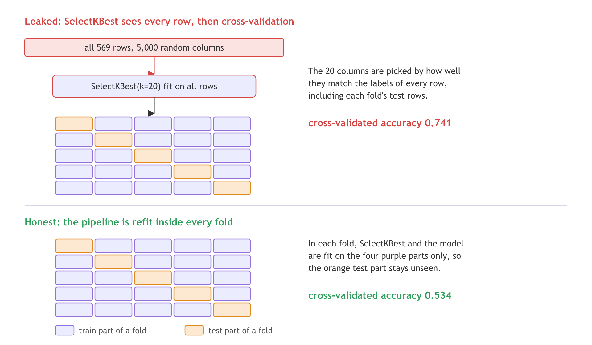
Always guessing benign is right 62.7% of the time. The leaked run claims 0.741 on pure noise, better than guessing, because among 5,000 random columns some match the labels of these 569 rows by chance, and the selection found them using the test folds too. Inside the pipeline, each fold picks its own 20 columns from its training part, and the score falls to 0.534: no better than chance, which is the truth.
The same mistake on the 30 real columns costs much less, because the strong columns win either way.
scaled = StandardScaler().fit_transform(X)      # the 30 real columns, scaled on all 569 rows
real_leaked = cross_val_score(LogisticRegression(), SelectKBest(k=5).fit_transform(scaled, y), y, cv=5)
real_honest = cross_val_score(make_pipeline(StandardScaler(), SelectKBest(k=5), LogisticRegression()),
                              X, y, cv=5)
print("real columns, leaked:", round(real_leaked.mean(), 3), " honest:", round(real_honest.mean(), 3))real columns, leaked: 0.951 honest: 0.949
Leaked 0.951 against honest 0.949: a gap of 0.002. A small gap on one dataset is no proof the habit is safe. The leak grows with the number of columns and shrinks with the number of rows, and real projects rarely know which case they are in.
Tuning on the test set
The third leak is choosing a hyperparameter by its test score. Below, 35 SVC settings are each scored on the test rows and the best one is kept.
from sklearn.metrics import f1_score

test_f1 = {}
for C in [0.001, 0.01, 0.1, 1, 10, 100, 1000]:
    for gamma in ["scale", 0.1, 0.01, 0.001, 0.0001]:
        model = make_pipeline(StandardScaler(), SVC(C=C, gamma=gamma)).fit(X_train, y_train)
        test_f1[(C, gamma)] = f1_score(y_test, model.predict(X_test))   # peeking at the test rows

picked = max(test_f1, key=test_f1.get)
print(len(test_f1), "settings, test f1 from", round(min(test_f1.values()), 3), "to", round(max(test_f1.values()), 3))
print("picked by the test rows:     C, gamma =", picked, " test f1", round(test_f1[picked], 3))
print("picked by cross-validation:", svc.best_params_, " test f1", round(f1_score(y_test, svc.predict(X_test)), 3))35 settings, test f1 from 0.771 to 0.987
picked by the test rows: C, gamma = (1000, 0.001) test f1 0.987
picked by cross-validation: {'svc__C': 1, 'svc__gamma': 0.01} test f1 0.975The test f1 ranges from 0.771 (C = 0.001 predicts benign for everything) to 0.987. Picking the top of 35 tries on 188 rows picks the setting that was luckiest on those rows, so 0.987 is no longer an estimate for new data: the test rows have become training data for the choice. The setting picked by cross-validation scores 0.975, and that is the honest SVC number.
What the leaked scores hid
- The deep tree: 1.000 leaked vs 0.904 honest. Scoring on training rows hides overfitting.
- Feature selection on random columns: 0.741 leaked vs 0.534 honest. Fitting a step on all rows lets the test folds pick the features.
- Tuning on the test rows: 0.987 picked vs 0.975 honest for SVC. Every look at the test set used for a decision makes its score more optimistic.
- The fix is the same each time: every step that learns from data sits inside the pipeline, every choice uses cross-validation on the training rows, and the test rows are used once.
Running the same workflow on California housing
Regression follows the same order. California housing has 20,640 districts and 8 features, and the target is the median house value in units of $100,000. The models are Multiple linear regression, Ridge regression and a random forest regressor, scored with R² as in R squared and adjusted R squared. A regression target is continuous, so there is no stratify.
The video's practical uses load_boston(), which scikit-learn removed in 1.2, and writes r2_score(y_pred, y_test). The code here uses fetch_california_housing() and the documented order r2_score(y_true, y_pred); the reversed order gives a different number.
from sklearn.datasets import fetch_california_housing
from sklearn.model_selection import train_test_split, cross_val_score
from sklearn.pipeline import make_pipeline
from sklearn.preprocessing import StandardScaler
from sklearn.linear_model import LinearRegression, Ridge
from sklearn.ensemble import RandomForestRegressor
from sklearn.metrics import r2_score

X, y = fetch_california_housing(return_X_y=True, as_frame=True)
X_train, X_test, y_train, y_test = train_test_split(X, y, test_size=0.33, random_state=42)

regressors = {"Linear regression": LinearRegression(), "Ridge": Ridge(alpha=1.0),
              "Random forest": RandomForestRegressor(random_state=42, n_jobs=-1)}
cv_r2 = {}
for name, model in regressors.items():
    cv_r2[name] = cross_val_score(make_pipeline(StandardScaler(), model),
                                  X_train, y_train, cv=5, scoring="r2").mean()
    print(f"{name:18} cv r2 {cv_r2[name]:.3f}")

best_name = max(cv_r2, key=cv_r2.get)           # chosen on the train rows only
best = make_pipeline(StandardScaler(), regressors[best_name]).fit(X_train, y_train)
print(best_name, "test r2:", round(r2_score(y_test, best.predict(X_test)), 3)) # y_true firstLinear regression cv r2 0.607 Ridge cv r2 0.607 Random forest cv r2 0.797 Random forest test r2: 0.804
What the regression run shows
- Linear regression and ridge both score about 0.607 in cross-validation. With 13,828 training rows and 8 features, the ridge penalty at α = 1 barely moves the weights.
- The random forest scores 0.797, because house value depends on location and income in ways a straight line cannot follow.
- The random forest's test R² is 0.804, close to its cross-validated score, so the train-only choice held up on new rows.
Leaked vs honest evaluation
| Step | Leaked | Honest |
|---|---|---|
| Scaling and feature selection | fit on all rows, then split or cross-validate | inside a pipeline, refit on the training part of every fold |
| Choosing a model or C | the best test score | the best cross-validated score on the training rows |
| Reporting the score | on the rows the model trained on | on the test rows, once |
| What the number means | how well the model fits data it has seen | how well it should do on new data |
| This lesson's run | 1.000 tree, 0.741 on noise, 0.987 SVC | 0.904 tree, 0.534 on noise, 0.975 SVC |
What this course left out
These topics sit next to the algorithms above and are the usual next steps.
| Topic | What it is | Where to go next |
|---|---|---|
| Feature engineering and EDA | Exploring the data with plots and statistics, then filling missing values, encoding categories and building new columns. | scikit-learn user guide, Preprocessing data and Imputation of missing values |
| Imbalanced data | Classes where one is rare (fraud, a rare disease). Beyond class_weight: resampling, threshold tuning, metrics such as average precision. | scikit-learn user guide, Tuning the decision threshold |
| ROC and AUC | A curve of true positive rate against false positive rate over every threshold; the area under it summarises a classifier in one number. | scikit-learn user guide, ROC |
| LDA | Linear discriminant analysis: a supervised dimensionality reduction that finds the directions that best separate the classes. | scikit-learn user guide, Linear and quadratic discriminant analysis |
| Time series | Data ordered in time, where a random split leaks the future into training; needs splits that respect time and forecasting models. | scikit-learn user guide, Time series split |
| Deployment | Saving a fitted pipeline and serving predictions from it in an app or an API. | scikit-learn user guide, Model persistence |
| Deep learning | Neural networks with many layers, for images, text and audio; the next subject after classical machine learning. | scikit-learn user guide, Neural network models, then a deep learning library |
Where you use the machine learning workflow
- Any new tabular problem, such as churn, loan approval or a diagnosis from measurements: compare several models on the training rows before picking one.
- Interviews and take-home tasks, where the question is often how you would evaluate a model, and the expected answer is a pipeline, cross-validation and a test set used once.
- Reviewing someone else's result: a score that is far above the cross-validated one, or near 1.000, is the first place to look for leakage.
SelectKBest, PCA, must be fitted on training rows only. Calling fit_transform on the whole X before train_test_split or cross_val_score leaks the test rows into it. Put the step in the pipeline and let fit handle it.Related
- Previous: Principal component analysis (PCA)
- Next: Machine Learning
- See also: Cross-validation, Hyperparameter tuning with GridSearchCV
- Reference: scikit-learn, Common pitfalls and recommended practices
- In the leakage example, change
k=20tok=100and run it again: compare how far the leaked and honest accuracies move apart. - Add
max_depth=4to the deep tree and print both accuracies again: the gap between the training and the test score should shrink. - Tune the random forest too: add
GridSearchCV(make_pipeline(StandardScaler(), RandomForestClassifier(random_state=42)), {"randomforestclassifier__n_estimators": [100, 300]}, scoring="f1", cv=5).fit(X_train, y_train)next to the two searches and check whether itsbest_score_beats logistic regression's 0.982.
Little by little, you're building something great.