R squared and adjusted R squared
R squared (R²) is a performance metric for regression that measures how much of the variation in the output a model explains, and adjusted R squared is a version that penalises extra features which do not help.
Last updated: 05 Oct, 2026 · scikit-learn 1.9.1
The cost function tells training which line is best. R² tells you afterwards how good that best line is, on a scale where 1 means perfect.
Comparing the best fit line with the mean line
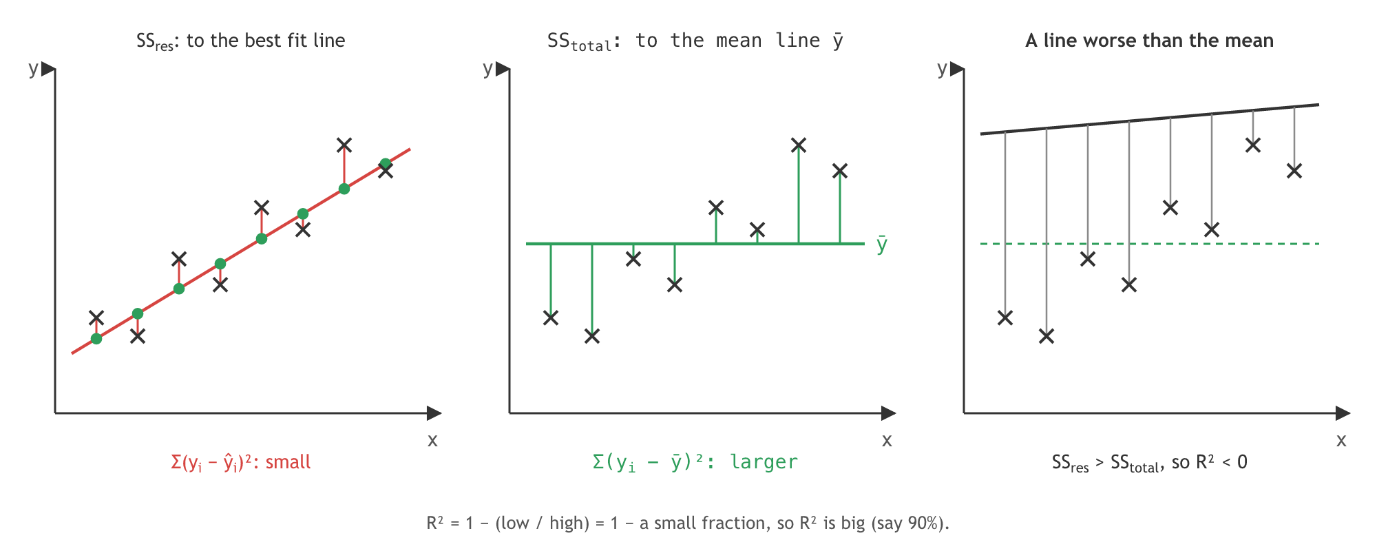
- SS_res, the sum of residuals, adds up the squared distances from each point to its predicted point on the best fit line.
- SS_total adds up the squared distances from each point to the mean line, a horizontal line at ȳ.
- The mean line is a worse fit, so SS_total is the higher number. Low divided by high is a small number, and 1 minus a small number is big: an R² of 90%, say, means the line fits well.
- R² can be negative, but only when the line is worse than the mean line, such as a line drawn above every point. A fitted line is at least as good as the mean, so this is rare.
Adding features that do not matter
Predict a house price. With bedrooms alone, say R² is 85%. Add location, which is correlated with price: R² rises to 90%. Now add gender, male or female, of the people living there. Gender has nothing to do with price, yet R² still creeps up, to 91%. Picking by R² alone would choose the 91% model, which carries a useless feature. Adjusted R² prevents that.
| Features | p | R² on the board |
|---|---|---|
| Bedrooms | 1 | 85% |
| Bedrooms, location | 2 | 90% |
| Bedrooms, location, gender | 3 | 91% |
Penalising extra predictors with adjusted R²
As p grows, N − p − 1 gets smaller, so the fraction gets bigger, and 1 minus it gets smaller. Unless the new feature raises R² enough to pay for itself, adjusted R² falls. The board's example: with p = 2, R² is 90% and adjusted R² 86%; with p = 3, R² rises to 91% while adjusted R² drops to 82%. Adjusted R² is always at or below R², which answers the video's interview question at the end of the clip: which of the two is bigger?
The board's 86% and 82% are illustrative values. They do not come from one N: with N = 8 houses the formula gives 86% for p = 2 and 84% for p = 3. The direction is the point: R² up, adjusted R² down.
Computing R² and adjusted R²
R² by hand and with r2_score
On the age and weight line from Simple linear regression, the formula and scikit-learn's r2_score should agree. A flat line at 80, above every point, shows a negative R².
import numpy as np
from sklearn.linear_model import LinearRegression
from sklearn.metrics import r2_score

age = np.array([[24], [25], [21], [27]])
weight = np.array([62, 63, 72, 62])
pred = LinearRegression().fit(age, weight).predict(age)

ss_res = np.sum((weight - pred) ** 2)
ss_total = np.sum((weight - weight.mean()) ** 2)
print("1 - SS_res / SS_total:  ", round(1 - ss_res / ss_total, 4))
print("r2_score(y_true, y_pred):", round(r2_score(weight, pred), 4))
print("a line above every point:", round(r2_score(weight, np.full(4, 80)), 2))1 - SS_res / SS_total: 0.7599 r2_score(y_true, y_pred): 0.7599 a line above every point: -13.15
Adjusted R² as a function
def adjusted_r2(r2, n, p):
    # n = number of data points, p = number of predictors
    return 1 - (1 - r2) * (n - 1) / (n - p - 1)
Checking the board's numbers
print("p = 2, R² = 0.90, N = 8:", round(adjusted_r2(0.90, n=8, p=2), 4))
print("p = 3, R² = 0.91, N = 8:", round(adjusted_r2(0.91, n=8, p=3), 4))p = 2, R² = 0.90, N = 8: 0.86 p = 3, R² = 0.91, N = 8: 0.8425
A house table with a useless column
The video gives no house table, so the rows here are generated: price depends on bedrooms and location plus noise, and gender is random.
import numpy as np
import pandas as pd

rng = np.random.default_rng(6)
n = 20
houses = pd.DataFrame({
    "bedrooms": rng.integers(1, 6, n),
    "location": rng.integers(1, 11, n),   # a 1-10 location score
    "gender": rng.integers(0, 2, n),      # who lives there: no link to the price
})
houses["price"] = 30 * houses.bedrooms + 5 * houses.location + rng.normal(0, 12, n)
Adding bedrooms, location and gender
from sklearn.linear_model import LinearRegression
from sklearn.metrics import r2_score

for cols in (["bedrooms"], ["bedrooms", "location"], ["bedrooms", "location", "gender"]):
    model = LinearRegression().fit(houses[cols], houses.price)
    r2 = r2_score(houses.price, model.predict(houses[cols]))
print(f"{' + '.join(cols):28} R² = {r2:.4f} adjusted R² = {adjusted_r2(r2, n, len(cols)):.4f}")bedrooms R² = 0.8112 adjusted R² = 0.8008 bedrooms + location R² = 0.9551 adjusted R² = 0.9499 bedrooms + location + gender R² = 0.9561 adjusted R² = 0.9478
What R² and adjusted R² printed
- The formula and r2_score agree on the age table: 0.7599. The line explains about three quarters of the variation in those four weights.
- The flat line at 80 scores −13.15: it is far worse than the mean line, so SS_res is 14 times SS_total.
- The board's numbers with N = 8 give 0.86 for p = 2, as the board says, and 0.8425 for p = 3, not 0.82.
- Location lifts both scores, R² from 0.8112 to 0.9551. Gender lifts R² by a hair (0.9551 to 0.9561) but lowers adjusted R² (0.9499 to 0.9478): the same pattern as the board's 90% to 91% and 86% to 82%.
R² vs adjusted R²
| R² | Adjusted R² | |
|---|---|---|
| Formula | 1 − SS_res / SS_total | 1 − (1 − R²)(N − 1) / (N − p − 1) |
| Adding a useless feature | Never goes down on the training data | Usually goes down |
| Size | The larger of the two | At or below R² |
| Use it to | Say how well one model fits | Compare models with different numbers of features |
| In scikit-learn | r2_score, model.score | No built-in; one line of Python |
Where you use R² and adjusted R²
- Reporting a regression model: R² on the test set says what share of the variation it explains.
- Feature selection: keep a new column only if adjusted R² goes up.
- Interviews: why R² keeps rising with useless features, and why adjusted R² is never larger.
r2_score takes the true values first: r2_score(y_true, y_pred). Swapping them gives a different number, because R² divides by the spread of whichever array comes first. Multiple linear regression shows the swap from the video's practical.Related
- Previous: Ordinary least squares
- Next: MSE, MAE and RMSE
- Reference: r2_score
- Change
n = 20ton = 200: with more rows the penalty for one extra feature shrinks, and the two numbers move closer. - Add a second random column,
rng.normal(size=n), as a fourth feature and run the loop with it: R² rises again and adjusted R² falls again. - Print
adjusted_r2(0.91, n=7, p=3): N = 7 is the house count that gives the board's 82%.
Every expert started right here.