Lasso regression
Lasso regression is a linear regression that adds λ times the sum of the absolute slopes to the cost function, which pushes some coefficients all the way to zero and so selects features.
Last updated: 05 Oct, 2026 · scikit-learn 1.9.1
Ridge regression squares the slopes. Lasso uses their absolute values instead, and that one change lets it drop features that do not help the prediction.
The board writes the penalty as |θ₀ + θ₁ + … + θₙ|, the absolute value of a sum; the Lasso penalty is the sum of the absolute values, |θ₁| + |θ₂| + … + |θₙ|, without θ₀.
Replacing slope squared with the absolute slope
Lasso is also called L1 regularization. The cost keeps the squared error (ŷ − y)² and adds λ times the "mode of slope", the modulus or absolute value |slope|, in place of slope squared.
With many features the hypothesis is ŷ = θ₀ + θ₁x₁ + θ₂x₂ + … + θₙxₙ, one slope per feature. As training goes on, the features that play no real role get a very small slope, and with the absolute value Lasso pushes it to exactly 0: "that entire feature is neglected". Squaring in Ridge makes a small slope's penalty tiny, so it shrinks but never vanishes; the absolute value keeps pushing at the same rate until it reaches 0. For example, ŷ = 0.52 + 0.65x₁ + 0.72x₂ + 0.34x₃ + 0.12x₄ might become ŷ = 0.52 + 0.51x₁ + 0.60x₂ + 0.14x₃ + 0·x₄ under Lasso: the weak slope 0.12 goes to 0 and x₄ drops out of the model.
So Lasso does two jobs: it prevents overfitting, and it performs feature selection. λ is again a hyperparameter, found with Cross-validation: try several λ values and keep the one that scores best. The video's advice is to try both regularizations and use whichever gives the better performance metric.
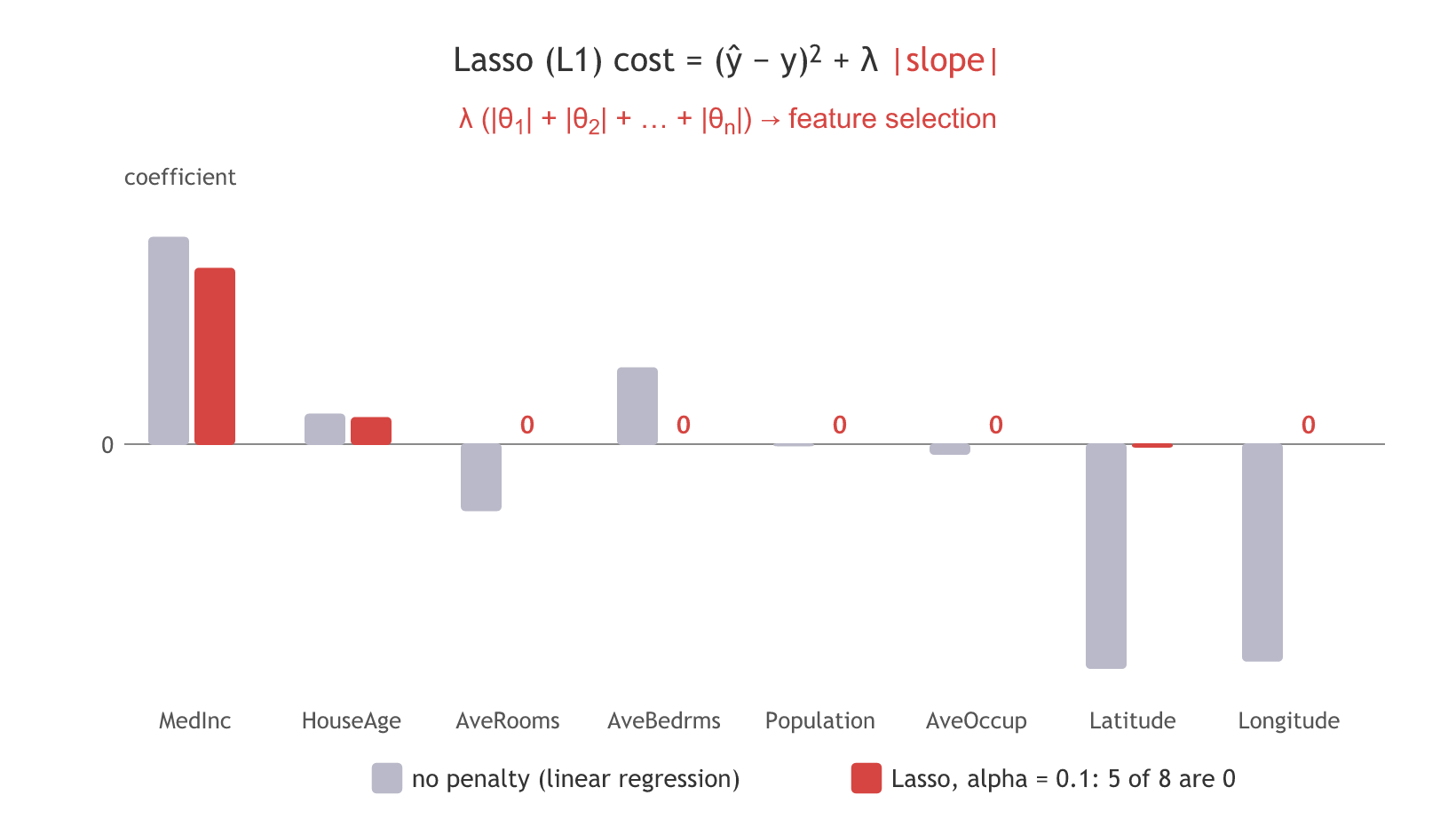
The bars above come from the run below: grey is linear regression on the scaled California features, red is Lasso with alpha 0.1.
Counting zero coefficients as alpha grows
The Lasso class
scikit-learn's Lasso minimises (1 / 2n) ‖y − Xw‖² + alpha ‖w‖₁, the mean squared error divided by 2 plus alpha times the sum of the absolute slopes. Because the error is averaged over the n rows, useful Lasso alphas are far smaller than Ridge alphas on the same data.
from sklearn.linear_model import Lasso

# alpha is λ; Lasso averages the squared error over the rows
lasso = Lasso(alpha=0.1)
lasso.fit(X, y)
print(lasso.coef_)            # some entries are exactly 0.0
Six alphas on California housing
import numpy as np
from sklearn.datasets import fetch_california_housing
from sklearn.preprocessing import StandardScaler
from sklearn.linear_model import Lasso

data = fetch_california_housing(as_frame=True)
X = StandardScaler().fit_transform(data.data)
y = data.target
names = np.array(data.feature_names)

for alpha in [0.001, 0.01, 0.05, 0.1, 0.5, 1]:
    coef = Lasso(alpha=alpha).fit(X, y).coef_
    zeros = int(np.sum(coef == 0))
print(f"alpha={alpha:<5} zeros={zeros} kept: {', '.join(names[coef != 0])}")alpha=0.001 zeros=0 kept: MedInc, HouseAge, AveRooms, AveBedrms, Population, AveOccup, Latitude, Longitude alpha=0.01 zeros=1 kept: MedInc, HouseAge, AveRooms, AveBedrms, AveOccup, Latitude, Longitude alpha=0.05 zeros=4 kept: MedInc, HouseAge, Latitude, Longitude alpha=0.1 zeros=5 kept: MedInc, HouseAge, Latitude alpha=0.5 zeros=7 kept: MedInc alpha=1 zeros=8 kept:
Which features Lasso keeps
- Small alpha keeps everything. At 0.001 no slope is 0; the fit is close to plain linear regression.
- The zeros grow with alpha. 1 zero at 0.01, 4 at 0.05, 5 at 0.1, 7 at 0.5 and all 8 at alpha 1, where the model predicts the same mean for every district.
- MedInc survives the longest. Median income is the last feature standing at alpha 0.5: of the eight, it carries the most information about the house value.
- Feature selection is a side effect of fitting. No separate step chooses the features; the zero slopes are part of the fitted model.
Pushing one slope to exactly 0
The two points (1, 2) and (2, 4) from Ridge regression show where the zeros come from. The Lasso cost is Σ(θ₁x − y)² + λ|θ₁|. For a positive slope its lowest point is at θ₁ = (20 − λ) / 10: slope 2 at λ = 0 and slope 1 at λ = 10. At λ = 20 the formula gives 0, and for any larger λ the lowest point stays at 0, where the absolute value puts a sharp corner in the curve.
The run draws the curves for λ = 0, 10, 20 and 40 and checks the slopes with scikit-learn. Lasso divides the squared error by 2n, which is 4 for two points, so its alpha is λ / 4.
import numpy as np
import matplotlib.pyplot as plt
from sklearn.linear_model import Lasso

x = np.array([1.0, 2.0])
y = np.array([2.0, 4.0])
theta1 = np.linspace(-0.2, 2.4, 261)

for lam, color in [(0, "black"), (10, "green"), (20, "orangered"), (40, "goldenrod")]:
    cost = np.array([np.sum((t * x - y) ** 2) + lam * abs(t) for t in theta1])
    print(f"lambda {lam:2}: lowest cost at slope {theta1[cost.argmin()]:.2f}")
    plt.plot(theta1, cost, color=color, label=f"lambda = {lam}")

for lam in [10, 20, 40]:
    lasso = Lasso(alpha=lam / 4, fit_intercept=False).fit(x.reshape(-1, 1), y)
    print(f"Lasso(alpha={lam}/4) slope: {lasso.coef_[0]:.3f}")

plt.title("Lasso cost for four values of lambda")
plt.xlabel("slope theta1")
plt.ylabel("J(theta1)")
plt.legend()
plt.show()lambda 0: lowest cost at slope 2.00 lambda 10: lowest cost at slope 1.00 lambda 20: lowest cost at slope 0.00 lambda 40: lowest cost at slope 0.00 Lasso(alpha=10/4) slope: 1.000 Lasso(alpha=20/4) slope: 0.000 Lasso(alpha=40/4) slope: 0.000
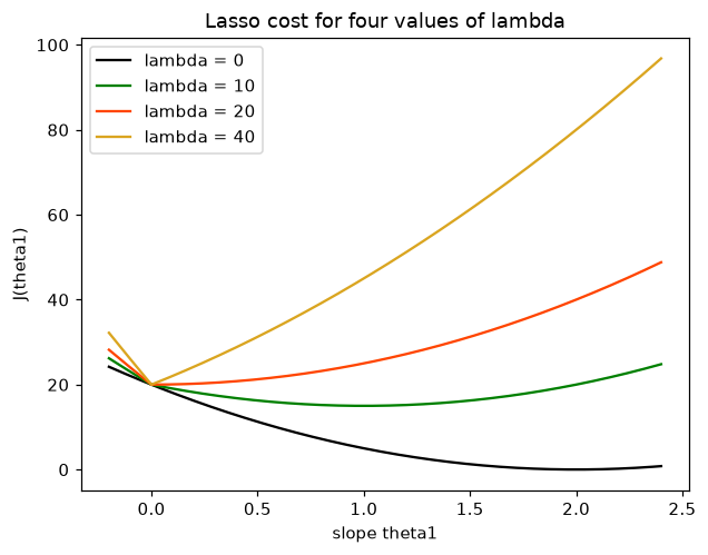
Where the slope hits 0
- λ = 10 halves the slope. The lowest cost moves from slope 2 to slope 1, and Lasso with alpha 10 / 4 gives the same 1.000.
- λ = 20 sets it to exactly 0. From here on the corner at 0 is the lowest point, so λ = 40 also gives 0.000.
- Ridge never gets there. On the same points Ridge's slope at λ = 30 is still 0.286; Lasso is at 0 from λ = 20.
Ridge vs Lasso
The video's summary, written as a table:
| Ridge regression | Lasso regression | |
|---|---|---|
| Also called | L2 regularization | L1 regularization |
| Penalty | λ Σ θⱼ² (slope squared) | λ Σ |θⱼ| (absolute slope) |
| Small slopes | shrink, never exactly 0 | pushed to exactly 0 |
| Two-point slope | 0.286 at λ = 30, never 0 | 0 from λ = 20 on |
| Purpose | prevent overfitting | prevent overfitting and feature selection |
| scikit-learn class | Ridge(alpha=...) | Lasso(alpha=...) |
Using both penalties at once is ElasticNet regression, which reduces overfitting and selects features in one model.
Where you use Lasso regression
- Many features, few that matter. Lasso finds the short list for you, as with MedInc and HouseAge above.
- A model people need to read. Three non-zero slopes are easier to explain than thirty.
- A first pass before another model. The features Lasso keeps are a reasonable starting set for a more complex model.
Related
- Previous: Ridge regression
- Next: ElasticNet regression
- Reference: scikit-learn: Lasso
- Add 0.2 and 0.3 to the alpha list and find the alpha where HouseAge drops out.
- Replace
Lasso(alpha=alpha)withRidge(alpha=alpha * 20640)(import Ridge from sklearn.linear_model) and count the zeros: there are none. - In the two-point run, change
[10, 20, 40]to[19, 21]: λ = 19 leaves a slope of (20 − 19) / 10 = 0.1, λ = 21 gives 0.
Slow is fine. Stopping is the only problem.