Ordinary least squares
Ordinary least squares (OLS) is a method that finds the intercept and slope of a linear regression line directly from a formula, by setting the derivatives of the squared error to zero instead of stepping towards the minimum.
Last updated: 05 Oct, 2026 · scikit-learn 1.9.1
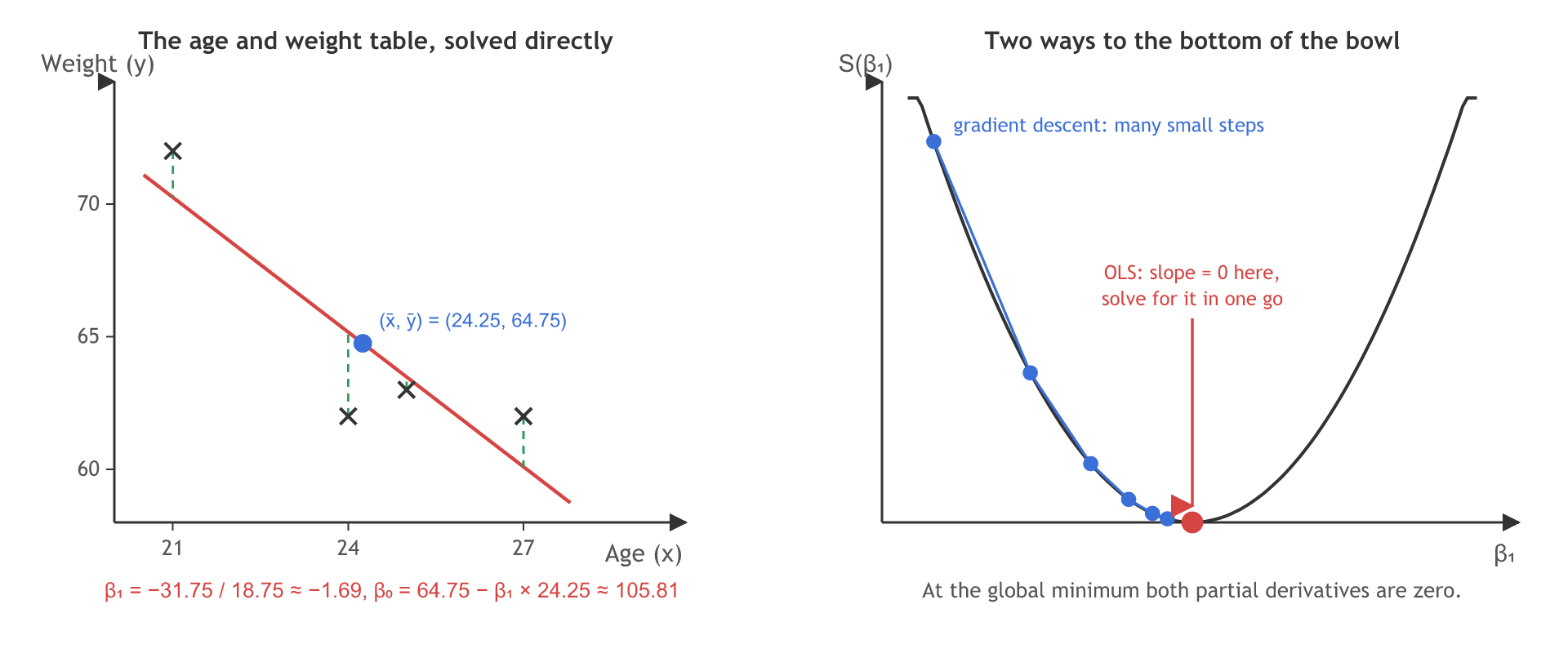
Gradient descent walks down the cost curve one small step at a time. The bottom of that curve is the one point where its slope is zero, so OLS solves for that point with algebra and lands there in one go.
Setting the slope of the error to zero
The notes write the line as hθ(x) = β₀ + β₁x, so ŷᵢ = β₀ + β₁xᵢ. The error to minimise is the mean squared error, called S here:
S is a bowl with one global minimum. At the minimum the slope is zero in both directions, so both partial derivatives are set to 0. Each one uses the rule that the derivative of a square, u², is 2u times the derivative of u:
Solving equation 1 for the intercept
Multiply equation 1 by −n/2, which leaves the sum equal to 0. Split the sum: Σyᵢ − nβ₀ − β₁Σxᵢ = 0. Move nβ₀ to the other side and divide by n. Σyᵢ/n is the mean ȳ and Σxᵢ/n is the mean x̄:
Solving equation 2 for the slope
Multiply equation 2 by −n/2 as well and put in β₀ = ȳ − β₁x̄. Each bracket becomes (yᵢ − ȳ) − β₁(xᵢ − x̄), still multiplied by xᵢ:
The deviations from a mean always add up to zero: Σ(yᵢ − ȳ) = 0 and Σ(xᵢ − x̄) = 0. So subtracting x̄ from the multiplier xᵢ changes nothing, and the xᵢ can be written as (xᵢ − x̄). Solving for β₁ gives the slope:
The notes drop the multiplier xᵢ midway and end with β₁ = Σ(yᵢ − ȳ) / Σ(xᵢ − x̄). Both of those sums are always 0, so that version cannot be computed; the slope needs the products (xᵢ − x̄)(yᵢ − ȳ) on top and the squares (xᵢ − x̄)² below, as above. The code further down prints both sums.
Working the formulas on the age and weight table
The notes end with a table to fill in: x, y, the deviations, then β₁ and β₀. On the video's table, x̄ = (24 + 25 + 21 + 27) / 4 = 24.25 and ȳ = (62 + 63 + 72 + 62) / 4 = 64.75:
| Age x | Weight y | x − x̄ | y − ȳ | (x − x̄)(y − ȳ) | (x − x̄)² |
|---|---|---|---|---|---|
| 24 | 62 | −0.25 | −2.75 | 0.6875 | 0.0625 |
| 25 | 63 | 0.75 | −1.75 | −1.3125 | 0.5625 |
| 21 | 72 | −3.25 | 7.25 | −23.5625 | 10.5625 |
| 27 | 62 | 2.75 | −2.75 | −7.5625 | 7.5625 |
| Sum | −31.75 | 18.75 |
These are the θ₁ ≈ −1.69 and θ₀ ≈ 105.81 that Simple linear regression printed and that Gradient descent reached after 575,671 steps.
Computing OLS in NumPy
The two formulas
import numpy as np

x = np.array([24, 25, 21, 27], dtype=float)   # age
y = np.array([62, 63, 72, 62], dtype=float)   # weight
x_bar, y_bar = x.mean(), y.mean()

beta1 = np.sum((x - x_bar) * (y - y_bar)) / np.sum((x - x_bar) ** 2)   # slope
beta0 = y_bar - beta1 * x_bar                                          # intercept
Matching LinearRegression
from sklearn.linear_model import LinearRegression

print("x̄ =", x_bar, " ȳ =", y_bar)
print("OLS by hand:      β1 =", round(beta1, 4), " β0 =", round(beta0, 4))
model = LinearRegression().fit(x.reshape(-1, 1), y)
print("LinearRegression: β1 =", round(model.coef_[0], 4), " β0 =", round(model.intercept_, 4))
print("the notes' sums: Σ(y − ȳ) =", np.sum(y - y_bar), " Σ(x − x̄) =", np.sum(x - x_bar))x̄ = 24.25 ȳ = 64.75 OLS by hand: β1 = -1.6933 β0 = 105.8133 LinearRegression: β1 = -1.6933 β0 = 105.8133 the notes' sums: Σ(y − ȳ) = 0.0 Σ(x − x̄) = 0.0
Reading the OLS run
- The hand formula and LinearRegression agree to four decimals: β₁ = −1.6933 and β₀ = 105.8133. scikit-learn's
LinearRegressionis ordinary least squares: its docs describe it as plain OLS (scipy.linalg.lstsq) wrapped as a predictor object. - x̄ = 24.25 and ȳ = 64.75 match the table above, and the line passes through that point.
- Both of the notes' sums print 0.0, which is why the products and squares are needed.
Ordinary least squares vs gradient descent
| Ordinary least squares | Gradient descent | |
|---|---|---|
| How it finds θ | Solves derivative = 0 with a formula | Repeats small steps down the slope |
| Learning rate | None | Needs α; too big diverges |
| Work on the age table | Two sums | 575,671 steps |
| With many features | Matrix algebra, slow when there are very many features | Scales to huge tables and neural networks |
| In scikit-learn | LinearRegression | SGDRegressor |
Where you use ordinary least squares
- Every
LinearRegressionfit in this course: the coefficients come from least squares, not from gradient descent. - Reading a regression report: the statsmodels library's
OLSprints the same coefficients with standard errors and p-values, as the practical notebooks do. - Interviews: derive β₀ = ȳ − β₁x̄ and the slope formula on paper, the way the notes do.
OLS adds no intercept unless you add a column of ones with sm.add_constant(X) (statsmodels OLS docs). The practical notebooks call sm.OLS(y_train, X_train) without it: the slope it prints, 17.2982, still matches LinearRegression, because the standardised weights average 0, but every prediction misses the 156.47 cm intercept and comes out near 0 (5.79 for a 75 kg person).Related
- Previous: Gradient descent
- Next: R squared and adjusted R squared
- Reference: Ordinary least squares in the scikit-learn user guide
- Add a fifth person, age 30 and weight 75, to
xandy: work out the new x̄ and ȳ, then check β₁ againstLinearRegression. - Run
np.polyfit(x, y, 1): it returns the same slope and intercept, in that order. - Replace the slope line with the notes' version,
np.sum(y - y_bar) / np.sum(x - x_bar), and read the result: 0 divided by 0 givesnan.
This is what real progress feels like.