Polynomial regression
Polynomial regression is a regression method that fits a curve by adding powers of the input feature, such as x² and x³, as new columns and then fitting an ordinary linear regression on them.
Last updated: 05 Oct, 2026 · scikit-learn 1.9.1
A straight line cannot follow points that bend. However well it is fitted, the best fit line of Simple linear regression leaves a large error on curved data; a curve brings the error down.
Fitting a curve with polynomial degrees
The notes start from a non-linear relationship: points that fall and then rise. The yellow straight line through them has a high error, and the curve through them a low one. Simple linear regression is hθ(x) = β₀ + β₁x and multiple linear regression hθ(x) = β₀ + β₁x₁ + β₂x₂ + β₃x₃. Polynomial regression keeps one input and raises it to powers, set by the degree:
- Degree 0: hθ(x) = β₀x⁰ = β₀, a constant value.
- Degree 1: hθ(x) = β₀x⁰ + β₁x¹, simple linear regression.
- Degree 2: hθ(x) = β₀x⁰ + β₁x¹ + β₂x², a parabola.
- Degree n: the powers continue up to βₙxⁿ.
It is still linear regression. x² is one more column of numbers, and the model is a weighted sum of its columns, linear in the β's. So the same least squares fit from Ordinary least squares finds the β's.
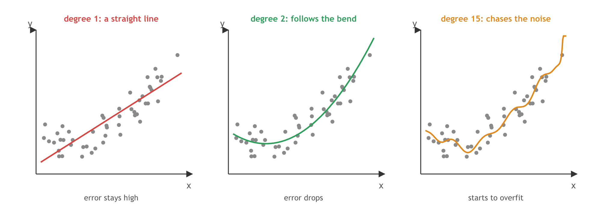
The degree is a value you choose. The notes draw degree 1 (a line), a curve of the right degree, and degree 15, which wiggles through every point and starts to overfit, the topic of Overfitting and underfitting.
Adding a second feature
With two independent features x₁ and x₂, degree 1 is hθ(x) = β₀ + β₁x₁ + β₂x₂. For degree 2 the notes write β₀ + β₁x₁ + β₂x₂ + β₃x₁² + β₄x₂². Degree 2 also includes the cross term x₁x₂, the product of the two features, and scikit-learn's PolynomialFeatures adds it, as the run below prints:
Fitting the notes' quadratic data
The practical notebook makes 100 points from the quadratic y = 0.5x² + 1.5x + 2 plus random noise, so the right answer is known. Its points are drawn without a seed, so its scores (0.626 for the line, 0.939 for degree 2) change on every run; with the seed here they repeat.
The curved data
import numpy as np
from sklearn.model_selection import train_test_split

rng = np.random.default_rng(42)
X = 6 * rng.random((100, 1)) - 3                                # 100 points between -3 and 3
y = 0.5 * X**2 + 1.5 * X + 2 + rng.standard_normal((100, 1))    # a curve plus noise
X_train, X_test, y_train, y_test = train_test_split(X, y, test_size=0.2, random_state=42)
Adding the powers with PolynomialFeatures
fit_transform on the training rows, then transform on the test rows, the same pattern as the scaler. include_bias=True adds the column of ones for x⁰.
from sklearn.preprocessing import PolynomialFeatures
from sklearn.linear_model import LinearRegression

poly = PolynomialFeatures(degree=2, include_bias=True)
X_train_poly = poly.fit_transform(X_train)   # columns 1, x, x²
X_test_poly = poly.transform(X_test)
regression = LinearRegression().fit(X_train_poly, y_train)
Recovering the curve's coefficients
from sklearn.metrics import r2_score

print("columns:", poly.get_feature_names_out())
print("first row:", X_train[0].round(3), "->", X_train_poly[0].round(3))
print("coefficients:", regression.coef_.round(3), " intercept:", regression.intercept_.round(3))
print("test R², degree 2:", round(r2_score(y_test, regression.predict(X_test_poly)), 4))

two = PolynomialFeatures(degree=2).fit(np.zeros((1, 2)))   # two input features
print("two features, degree 2:", two.get_feature_names_out(["x1", "x2"]))columns: ['1' 'x0' 'x0^2'] first row: [1.684] -> [1. 1.684 2.837] coefficients: [[0. 1.54 0.498]] intercept: [2.076] test R², degree 2: 0.9001 two features, degree 2: ['1' 'x1' 'x2' 'x1^2' 'x1 x2' 'x2^2']
A pipeline for any degree
The notebook wraps the two steps in a Pipeline, so one fit call adds the powers and fits the line. A scaler between them keeps high powers in a range the fit handles well.
from sklearn.pipeline import Pipeline
from sklearn.preprocessing import StandardScaler

def poly_regression(degree):
    return Pipeline([
        ("poly_features", PolynomialFeatures(degree=degree, include_bias=True)),
        ("scaler", StandardScaler()),       # x to the 15th reaches millions: scale the columns
        ("lin_reg", LinearRegression()),
    ])
Comparing degrees 1, 2, 3 and 15
import matplotlib.pyplot as plt

X_new = np.linspace(-3, 3, 200).reshape(200, 1)
plt.plot(X_train, y_train, "b.", label="training points")
plt.plot(X_test, y_test, "g.", label="testing points")
for degree, color in [(1, "orange"), (2, "red"), (3, "black"), (15, "purple")]:
    model = poly_regression(degree).fit(X_train, y_train)
    train_r2 = r2_score(y_train, model.predict(X_train))
    test_r2 = r2_score(y_test, model.predict(X_test))
    print(f"degree {degree:>2}: train R² {train_r2:.3f}, test R² {test_r2:.3f}")
    plt.plot(X_new, model.predict(X_new), color=color, label=f"degree {degree}")
plt.axis([-4, 4, 0, 10])
plt.title("Polynomial regression by degree")
plt.xlabel("X")
plt.ylabel("y")
plt.legend(loc="upper left")
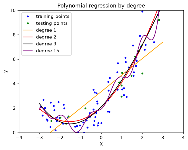
plt.show()degree 1: train R² 0.658, test R² 0.827 degree 2: train R² 0.861, test R² 0.900 degree 3: train R² 0.864, test R² 0.911 degree 15: train R² 0.887, test R² 0.879
Reading the degrees
- Degree 2 recovers the curve. The columns are 1, x and x², and the coefficients come out near the true 1.5 and 0.5 with an intercept near 2. The first coefficient is 0 because the column of ones is already covered by the intercept.
- Two features give six columns at degree 2: 1, x1, x2, x1², x1·x2 and x2², the cross term included.
- The line scores worst, and degree 2 jumps ahead on both the training and the test rows. Degree 3 adds a little; the true curve has degree 2.
- Degree 15 scores highest on the training rows and lower on the test rows than degrees 2 and 3: it has started to fit the noise. With fewer points the gap grows much wider.
Polynomial regression vs linear regression
| Linear regression | Polynomial regression | |
|---|---|---|
| Shape of the fit | A straight line or plane | A curve |
| Columns the model sees | x | 1, x, x², …, xⁿ |
| Choice to make | None | The degree |
| Risk | Underfits curved data | Overfits when the degree is too high |
| In scikit-learn | LinearRegression | PolynomialFeatures + LinearRegression in a Pipeline |
Where you use polynomial regression
- Curved relationships with one or two inputs, such as growth that speeds up over time.
- Interaction effects: the x₁x₂ column lets the effect of one feature depend on the other.
- A step before regularisation: many polynomial columns plus Ridge regression keeps a flexible curve from overfitting.
Related
- Previous: Multiple linear regression
- Next: Cross-validation
- See also: Overfitting and underfitting
- Reference: PolynomialFeatures
- Change both
(100, 1)sizes to(30, 1): degree 15's training R² stays high while its test R² falls far below zero. - Set
include_bias=Falseinpoly: the column of ones disappears and the coefficients keep their values. - Print
PolynomialFeatures(degree=3).fit(np.zeros((1, 10))).n_output_features_to check the 286 columns.
Slow is fine. Stopping is the only problem.