Linear regression assumptions
Linear regression assumptions are the conditions on the data under which a linear regression trains well and its slopes can be trusted: roughly normal features, scaled features, a linear relationship and no multicollinearity.
Last updated: 05 Oct, 2026 · scikit-learn 1.9.1
A linear regression always returns a line, even when a line is the wrong shape for the data. These checks, from the end of the video's regression session, say when to trust it.
Checking the four assumptions
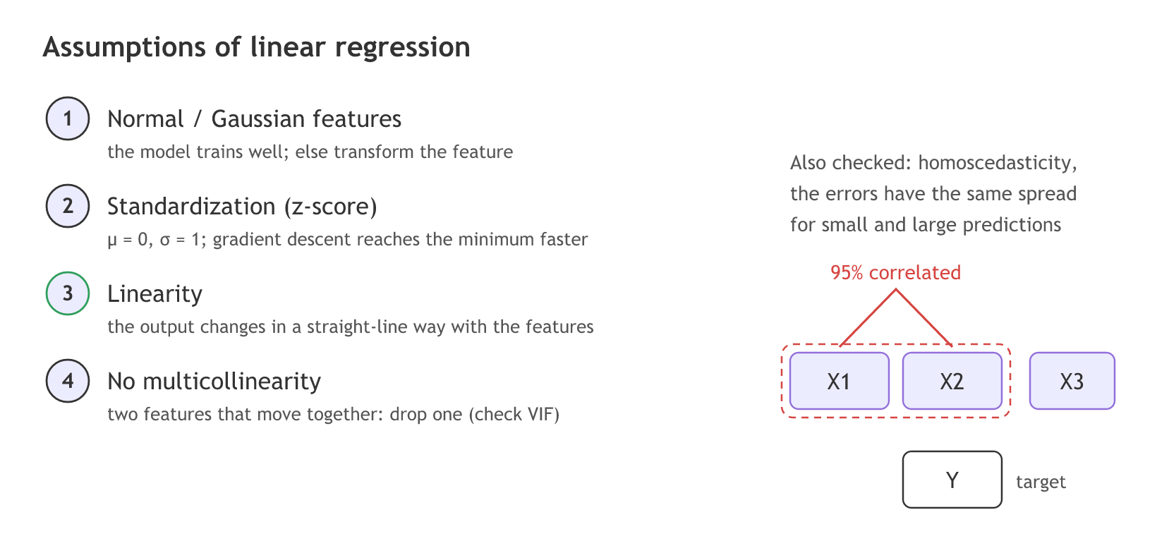
Normal features and feature transformation
If the features follow a normal (Gaussian) distribution, the model trains well. If a feature does not, apply a mathematical function to it to bring it closer to normal, which the video calls feature transformation; taking the log of a long-tailed feature is the usual one. Strictly, the classical assumption is about the errors of the fit being normal, not the features; normal-looking features help, but they are not required.
Standardization with the z-score
Standardization (the StandardScaler) rescales a feature with the z-score so its mean μ becomes 0 and its standard deviation σ becomes 1. Wherever gradient descent is involved, it helps: on scaled data the cost surface is closer to round, and the steps reach the global minimum quickly instead of zig-zagging across a long valley. It is not compulsory, but it makes training faster.
Linearity
Linear regression works well when the output changes in a straight-line way with each feature. If the relationship bends, a straight line underfits; polynomial features (as in Overfitting and underfitting) or another model are the fix.
Multicollinearity and VIF
Multicollinearity means two features move together. In the video's sketch X1 and X2 are 95% correlated. Using both adds little: "we can drop this particular feature" and keep one. The variance inflation factor (VIF) measures it per feature: fit the feature from all the other features, take that R², and compute 1 / (1 − R²). A VIF of 1 means no overlap; values above about 5 to 10 are usually treated as a problem.
The video also names homoscedasticity: the errors should have about the same spread for small and large predictions. A plot of the residuals against the predicted values shows it; a funnel shape, narrow on one side and wide on the other, means the assumption fails.
Checking the assumptions on California housing
StandardScaler
fit learns μ and σ of each column, transform applies the z-score; fit_transform does both.
from sklearn.preprocessing import StandardScaler

scaler = StandardScaler()
X_scaled = scaler.fit_transform(X)    # each column: (x - mean) / std
print(scaler.mean_, scaler.scale_)    # the μ and σ it learned
Skew and the z-score
Skew measures how lopsided a distribution is: 0 is symmetric, a large positive value is a long right tail. The first lines check one feature against the normal assumption; the rest compute the z-score by hand and with StandardScaler.
import numpy as np
from sklearn.datasets import fetch_california_housing
from sklearn.preprocessing import StandardScaler

X, y = fetch_california_housing(return_X_y=True, as_frame=True)

# assumption 1: is the feature close to normal? skew 0 = symmetric
print("Population skew:", round(X["Population"].skew(), 2))
print("log(1 + Population) skew:", round(np.log1p(X["Population"]).skew(), 2))

# assumption 2: z = (x - mu) / sigma, by hand and with StandardScaler
income = X["MedInc"]
mu, sigma = income.mean(), income.std(ddof=0)
by_hand = (income - mu) / sigma
scaled = StandardScaler().fit_transform(X[["MedInc"]])[:, 0]
print("mu =", round(mu, 3), " sigma =", round(sigma, 3))
print("first three z by hand:", by_hand[:3].round(3).tolist())
print("first three z scaler: ", scaled[:3].round(3).tolist())
print("after scaling: mean", abs(round(scaled.mean(), 3)), " std", round(scaled.std(), 3))Population skew: 4.94 log(1 + Population) skew: -1.04 mu = 3.871 sigma = 1.9 first three z by hand: [2.345, 2.332, 1.783] first three z scaler: [2.345, 2.332, 1.783] after scaling: mean 0.0 std 1.0
Correlation and VIF with numpy
For standardized features the VIF of every column is on the diagonal of the inverse of the correlation matrix, so numpy computes all of them in one line. The last lines check one value the long way, with a LinearRegression of AveRooms on the other seven features.
import numpy as np
import pandas as pd
from sklearn.datasets import fetch_california_housing
from sklearn.linear_model import LinearRegression

X, y = fetch_california_housing(return_X_y=True, as_frame=True)

corr = X.corr()
print("AveRooms vs AveBedrms:", round(corr.loc["AveRooms", "AveBedrms"], 2))
print("Latitude vs Longitude:", round(corr.loc["Latitude", "Longitude"], 2))

# VIF of every feature = the diagonal of the inverse correlation matrix
vif = pd.Series(np.diag(np.linalg.inv(corr.to_numpy())), index=X.columns)
print(vif.round(2))

# the same number for AveRooms, from its R2 against the other features
others = X.drop(columns=["AveRooms"])
r2 = LinearRegression().fit(others, X["AveRooms"]).score(others, X["AveRooms"])
print("1 / (1 - R2) for AveRooms:", round(1 / (1 - r2), 2))

# drop one feature of the correlated pair and recompute
X_small = X.drop(columns=["AveBedrms"])
vif_small = pd.Series(np.diag(np.linalg.inv(X_small.corr().to_numpy())), index=X_small.columns)
print("AveRooms VIF after dropping AveBedrms:", round(vif_small["AveRooms"], 2))AveRooms vs AveBedrms: 0.85 Latitude vs Longitude: -0.92 MedInc 2.50 HouseAge 1.24 AveRooms 8.34 AveBedrms 6.99 Population 1.14 AveOccup 1.01 Latitude 9.30 Longitude 8.96 dtype: float64 1 / (1 - R2) for AveRooms: 8.34 AveRooms VIF after dropping AveBedrms: 1.26
What the checks found
- Population is far from normal. A skew of 4.94, a long right tail of crowded districts. log(1 + x) brings it to −1.04, much closer to symmetric: the feature transformation the video describes.
- StandardScaler is the z-score. With μ = 3.871 and σ = 1.9, the first incomes become 2.345, 2.332 and 1.783 both by hand and with the scaler, and the scaled column has mean 0 and standard deviation 1.
- AveRooms and AveBedrms are the video's X1 and X2. They are 0.85 correlated, and their VIFs are 8.34 and 6.99. The long way gives the same 8.34 for AveRooms.
- Dropping one fixes the other. Without AveBedrms, the VIF of AveRooms falls from 8.34 to 1.26.
- Latitude and Longitude also score high, 9.30 and 8.96, with a correlation of −0.92. They are a different case: together they locate a district, so dropping one would lose information.
Assumption checks vs fixes
| Assumption | How to check | If it fails |
|---|---|---|
| Normal features (normal errors) | skew, a histogram, a residual histogram | transform the feature, for example log(1 + x) |
| Scaled features | mean and standard deviation of each column | StandardScaler |
| Linearity | scatter plot of each feature against y | polynomial features or a non-linear model |
| No multicollinearity | correlation matrix, VIF above about 5 to 10 | drop one of the pair, or use Ridge |
| Homoscedasticity | residuals against predictions: no funnel | transform the target, for example log(y) |
Where you use these checks
- Before trusting the slopes. With high VIF the individual coefficients swing from sample to sample, even when the predictions stay fine.
- Before gradient descent or regularization. Scaling makes training faster and makes one alpha mean the same for every slope.
- When the fit is poor. A low R² on a curved relationship points to the linearity assumption, not to the algorithm.
Related
- Previous: Hyperparameter tuning with GridSearchCV
- Next: Logistic regression
- Reference: scikit-learn: Standardization
- Print the skew of
X["MedInc"]and ofnp.log1p(X["MedInc"]). - Drop
Latitudeinstead of AveBedrms and recompute the VIF table: Longitude's VIF falls close to 1. - Replace StandardScaler with
MinMaxScalerfrom sklearn.preprocessing and print the minimum and maximum of the scaled column.
Little by little, you're building something great.