Support vector regression (SVR)
Support vector regression (SVR) is the regression form of the support vector machine that fits a line with a tube of width ε around it and counts only the points outside the tube as errors.
Last updated: 05 Oct, 2026 · scikit-learn 1.9.1
Support vector machines (SVM) separated two classes with the widest margin. SVR turns the margin around: the points should fall inside it. Linear regression pays for every residual, however small; SVR pays nothing for an error smaller than ε.
Drawing the ε tube around the line
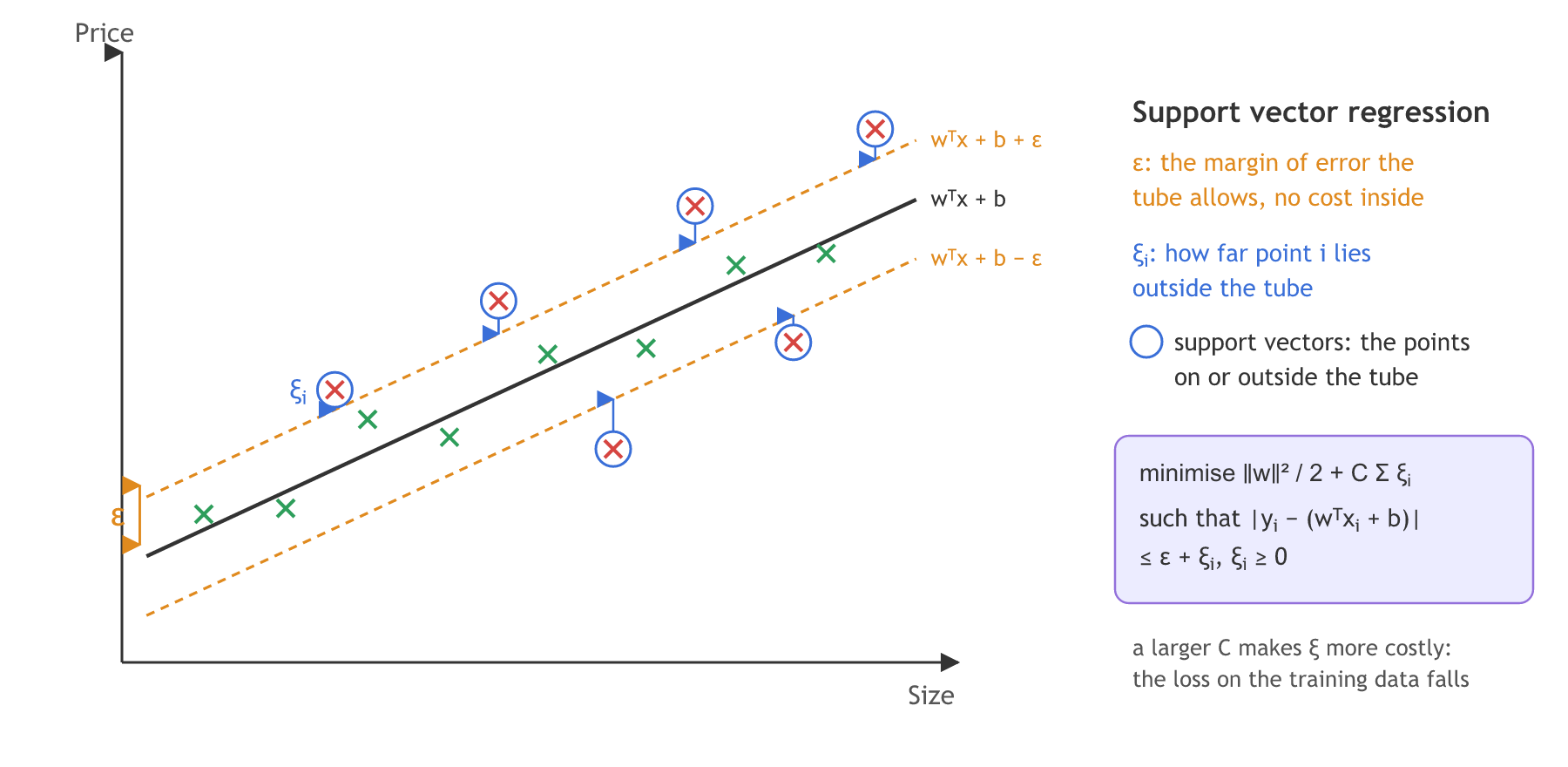
The worked example predicts a house price from its size. SVR draws the best fit line wᵀx + b, the same hyperplane equation as the classifier, and two marginal lines parallel to it, wᵀx + b + ε above and wᵀx + b − ε below. ε (epsilon) is the margin of error: a prediction within ε of the true price costs nothing.
Some points fall outside the tube. For each of them, ξᵢ (xi, the slack) is its distance past the edge of the tube, the error above the margin. The points on or outside the tube are the support vectors: they decide where the line goes, and the points inside the tube do not.
Writing the SVR cost function
The cost function has the same two parts as the soft margin SVM: keep w small, and pay C for every unit of slack. The constraint says each point is within ε of the line, plus its own slack ξᵢ.
The board writes ‖w‖/2 and |yᵢ − wᵢxᵢ|; the standard form squares the norm, as in the classifier, and keeps b inside the absolute value. Each point's slack is its ε-insensitive loss, zero inside the tube and growing in a straight line outside it. It plays the part the hinge loss plays for the classifier.
C is a hyperparameter. A larger C makes slack more expensive, so the line bends toward the points outside the tube and the loss on the training data falls; too large a C fits noise.
Fitting SVR on ten house sizes
Ten houses, size in hundreds of square feet and price in lakhs, with a tube of ε = 3.
A linear SVR with ε = 3
kernel="linear" gives a straight line. epsilon is the half width of the tube, in the units of the target. After fitting, coef_ holds w, intercept_ holds b and support_ the row numbers of the support vectors.
from sklearn.svm import SVR

svr = SVR(kernel="linear", C=10, epsilon=3).fit(size, price)
residual = price - svr.predict(size)
loss = np.maximum(0, np.abs(residual) - 3) # the epsilon-insensitive lossimport numpy as np
from sklearn.svm import SVR
size = np.array([1, 2, 3, 4, 5, 6, 7, 8, 9, 10]).reshape(-1, 1) # hundreds of square feet
price = np.array([12, 15, 23, 19, 26, 30, 28, 36, 34, 45]) # lakhs
svr = SVR(kernel="linear", C=10, epsilon=3).fit(size, price)
print("w:", svr.coef_[0].round(3), " b:", svr.intercept_.round(3))
residual = price - svr.predict(size)
print("residuals:", residual.round(2))
print("support vectors (house numbers):", svr.support_ + 1)
print("epsilon-insensitive loss:", np.maximum(0, np.abs(residual) - 3).round(2))w: [3.] b: [10.] residuals: [-1. -1. 4. -3. 1. 2. -3. 2. -3. 5.] support vectors (house numbers): [ 3 4 7 9 10] epsilon-insensitive loss: [0. 0. 1. 0. 0. 0. 0. 0. 0. 2.]
What the tube fit shows
- The line is price = 3 × size + 10 (w = 3, b = 10).
- Five houses are support vectors, numbers 3, 4, 7, 9 and 10: their residuals, 4, −3, −3, −3 and 5, are at least ε = 3 in size. Houses 4, 7 and 9 sit exactly on the edge of the tube.
- Only houses 3 and 10 have a loss, 1 and 2, the part of their error beyond ε. The five houses inside the tube cost nothing and do not shape the line.
Predicting the total bill on the tips dataset
The tips dataset has 244 restaurant bills with the tip, the customer's sex, smoker or not, the day, lunch or dinner, and the size of the party. The task is to predict the total bill. sns.load_dataset downloads it once.
Encoding the columns and fitting SVR
The four text columns become 0 or 1 columns with pd.get_dummies. SVR() uses the rbf kernel by default, with C=1 and epsilon=0.1.
df = sns.load_dataset("tips")
X = pd.get_dummies(df[["tip", "sex", "smoker", "day", "time", "size"]], drop_first=True,
                   columns=["sex", "smoker", "day", "time"]).astype(float)
y = df["total_bill"]
svr = SVR().fit(X_train, y_train)
Tuning C and gamma with GridSearchCV
gamma sets how far one point's influence reaches in the rbf kernel. Hyperparameter tuning with GridSearchCV tries every pair from the grid with 5-fold cross-validation.
param_grid = {"C": [0.1, 1, 10, 100, 1000], "gamma": [1, 0.1, 0.01, 0.001, 0.0001], "kernel": ["rbf"]}
grid = GridSearchCV(SVR(), param_grid, cv=5).fit(X_train, y_train)
grid.best_params_import pandas as pd
import seaborn as sns
from sklearn.model_selection import train_test_split, GridSearchCV
from sklearn.svm import SVR
from sklearn.metrics import r2_score, mean_absolute_error
df = sns.load_dataset("tips")
X = pd.get_dummies(df[["tip", "sex", "smoker", "day", "time", "size"]], drop_first=True,
columns=["sex", "smoker", "day", "time"]).astype(float)
y = df["total_bill"]
X_train, X_test, y_train, y_test = train_test_split(X, y, test_size=0.25, random_state=10)
svr = SVR().fit(X_train, y_train)
pred = svr.predict(X_test)
print(f"default SVR: R2 {r2_score(y_test, pred):.3f} MAE {mean_absolute_error(y_test, pred):.3f}")
print("support vectors:", len(svr.support_), "of", len(X_train))
param_grid = {"C": [0.1, 1, 10, 100, 1000], "gamma": [1, 0.1, 0.01, 0.001, 0.0001], "kernel": ["rbf"]}
grid = GridSearchCV(SVR(), param_grid, cv=5).fit(X_train, y_train)
pred = grid.predict(X_test)
print("best:", grid.best_params_)
print(f"tuned SVR: R2 {r2_score(y_test, pred):.3f} MAE {mean_absolute_error(y_test, pred):.3f}")default SVR: R2 0.462 MAE 4.117
support vectors: 180 of 183
best: {'C': 1000, 'gamma': 0.0001, 'kernel': 'rbf'}
tuned SVR: R2 0.508 MAE 3.868What the tips models show
- The default SVR scores a test R² of 0.462, with a mean absolute error of 4.117 dollars.
- 180 of the 183 training bills are support vectors: the default ε = 0.1 dollars is so narrow that almost every bill falls outside the tube.
- The grid picks C = 1000 and gamma = 0.0001, a smooth rbf kernel with expensive errors, and the test R² rises to 0.508 with an error of 3.868 dollars.
SVR vs linear regression
| SVR | Linear regression | |
|---|---|---|
| Which errors cost | only those larger than ε | every residual |
| How an error costs | in a straight line past ε (ε-insensitive loss) | squared |
| Points that shape the fit | the support vectors, on or outside the tube | every training point |
| Curved relationships | kernels (rbf, polynomial) | only by adding features by hand |
| Settings to tune | C, epsilon, kernel and gamma | none for plain least squares |
Where you use support vector regression
- Small and medium tabular datasets, such as the 244 tips, where a curved fit helps and training time is not a problem.
- Data with a few large errors, which the straight-line loss outside the tube punishes less than squared error does.
- A known tolerance: when an error of up to ε does not matter, such as a price quoted to the nearest lakh.
epsilon is measured in the target's units, and its default of 0.1 is tiny for a bill in dollars and meaningless for a price in rupees. Pick ε from the size of error you can accept, and tune C and gamma: on the tips data the defaults gave a lower R² than the grid's choice.Related
- Previous: Support vector machines (SVM)
- Next: SVM kernels
- See also: Simple linear regression
- Reference: SVR in the scikit-learn API
- Change
epsilon=3toepsilon=6on the ten houses and count the support vectors. - Set
C=0.01on the ten houses and compare w with the run above. - Fit
SVR(kernel="linear")on the tips data and compare its test R² with the tuned rbf model.
Slow is fine. Stopping is the only problem.