SVM kernels
An SVM kernel is a function that lets a support vector machine separate data that no straight line can split, by working as if the points had been moved into a higher dimension.
Last updated: 05 Oct, 2026 · scikit-learn 1.9.1
Support vector machines (SVM) drew a straight hyperplane. When one class sits inside the other, every straight line fails, and a kernel is the way out.
Moving the points into a higher dimension
The video starts from a dataset that is not linearly separable: one class in the middle, the other around it. Any best fit line leaves many points on the wrong side. An SVM kernel converts the data from two dimensions into three: the middle points are raised, the outer points stay low, and a plane divides them.
The transformation from a lower dimension to a higher one is done with a mathematical formula, and each kind of kernel has its own: polynomial, rbf (radial basis function) and sigmoid.
Squaring one feature to separate one dimension
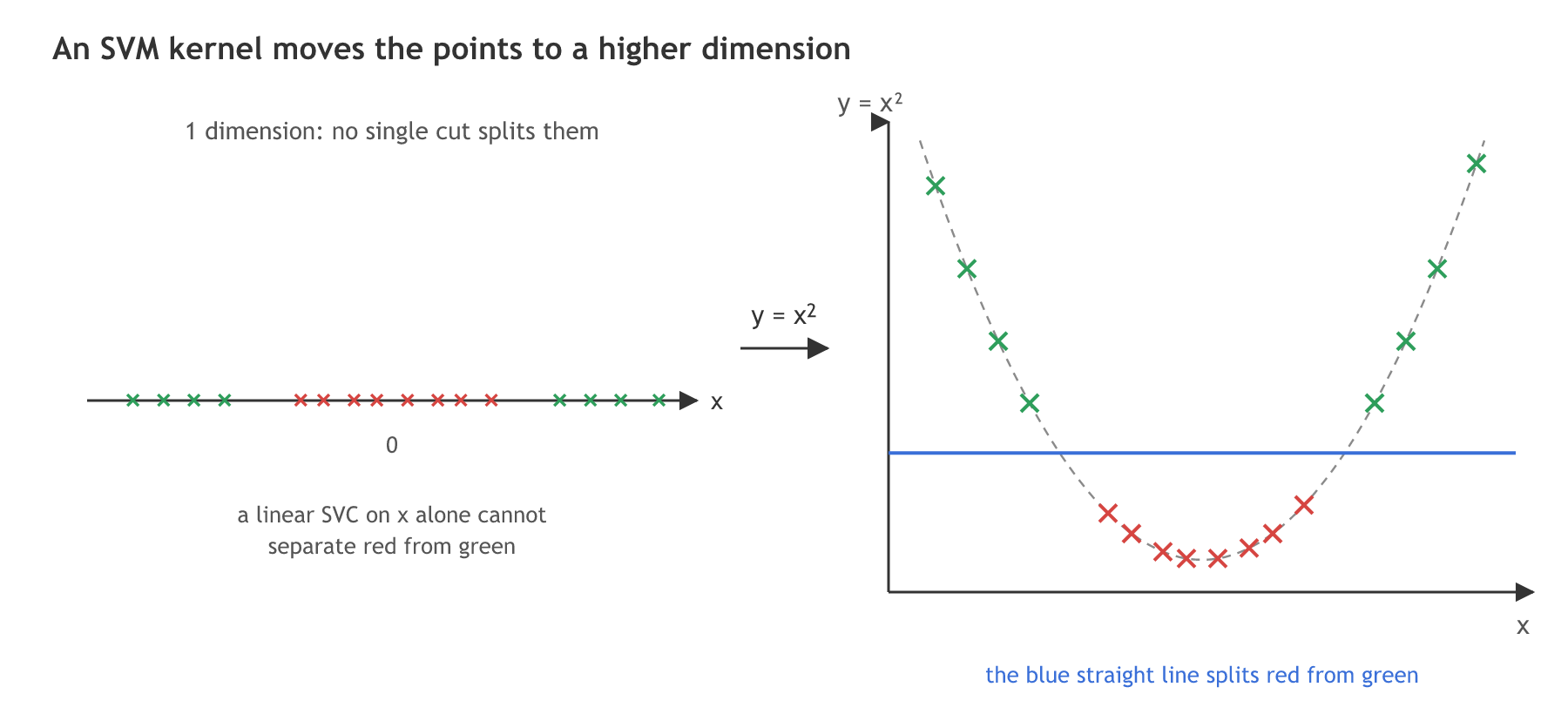
The simplest case has one feature x. The points of one class sit near 0, the points of the other class on both sides of them. A single cut on x leaves errors whichever way it goes. The video applies y = f(x) = x² to every point (the data is centred at 0). The points now lie on a parabola: the middle class low, the outer class high, and a straight line separates them.
The same idea works in any number of dimensions: two dimensions go to three, three to four, and so on.
Adding x² as a second feature
import numpy as np
from sklearn.svm import SVC

x = np.array([-3.4, -3.0, -2.6, -2.2, -1.2, -0.9, -0.5, -0.2, 0.2, 0.6, 0.9, 1.3, 2.2, 2.6, 3.0, 3.5])
y = np.array([0, 0, 0, 0, 1, 1, 1, 1, 1, 1, 1, 1, 0, 0, 0, 0])     # 1 = the middle class

one_d = x.reshape(-1, 1)
two_d = np.c_[x, x ** 2]                                            # add y = x squared
print("linear SVC on x:        accuracy", SVC(kernel="linear").fit(one_d, y).score(one_d, y))
print("linear SVC on x and x^2: accuracy", SVC(kernel="linear").fit(two_d, y).score(two_d, y))linear SVC on x: accuracy 0.6875 linear SVC on x and x^2: accuracy 1.0
The linear SVC on x alone gets 0.6875 of the 16 points right (11 of them), the best a single cut can do. With x² added as a second feature it gets every point right.
Expanding the polynomial kernel
For two features x₁ and x₂ the video writes the polynomial kernel as the vector product of the points plus 1, raised to the power d. Working out the product gives the terms x₁², x₂² and x₁x₂ next to x₁ and x₂. Keeping each term once, the two dimensions become five features: x₁, x₂, x₁², x₂² and x₁x₂, and in that space a plane can split the classes.
A kernel takes two points, not one. For d = 2 and c = 1, (aᵀb + 1)² equals the dot product of the two points after each is mapped to (x₁², x₂², √2·x₁x₂, √2·x₁, √2·x₂, 1). The SVM only ever needs those dot products, so the kernel gives the answer without building the new columns. That shortcut is called the kernel trick.
Training a linear SVC on the polynomial features
Plotted with x₁², x₂² and x₁x₂ as the axes, the points of the two classes separate, so a linear SVC finds a plane between them. Selecting kernel="poly" does the same work internally, and the choice between the polynomial, rbf and sigmoid kernels is a hyperparameter, tuned like any other.
The example takes 100 heights between −5 and 5. At each height it places a point on a circle of radius 5 on both sides, which draws the whole inner circle, and a point on a circle of radius 10 on both sides, which draws two arcs to the left and right of it. The inner circle is class 1, the arcs class 0.
The circle and the two arcs
x = np.linspace(-5.0, 5.0, 100)                    # 100 heights between -5 and 5
outer = np.sqrt(10 ** 2 - x ** 2)                  # on a circle of radius 10: two arcs
inner = np.sqrt(5 ** 2 - x ** 2)                   # on a circle of radius 5: the whole circle
X = np.vstack([np.c_[np.hstack([outer, -outer]), np.hstack([x, -x])],
               np.c_[np.hstack([inner, -inner]), np.hstack([x, -x])]])
y = np.r_[np.zeros(200), np.ones(200)]             # 0 = the arcs, 1 = the inner circle
The polynomial features by hand
Xp = np.c_[X, X[:, 0] ** 2, X[:, 1] ** 2, X[:, 0] * X[:, 1]]    # x1, x2, x1^2, x2^2, x1*x2
SVC(kernel="linear").fit(Xp_train, y_train).score(Xp_test, y_test)import numpy as np
import matplotlib.pyplot as plt
from sklearn.model_selection import train_test_split
from sklearn.svm import SVC
x = np.linspace(-5.0, 5.0, 100) # 100 heights between -5 and 5
outer = np.sqrt(10 ** 2 - x ** 2) # on a circle of radius 10: two arcs
inner = np.sqrt(5 ** 2 - x ** 2) # on a circle of radius 5: the whole circle
X = np.vstack([np.c_[np.hstack([outer, -outer]), np.hstack([x, -x])],
np.c_[np.hstack([inner, -inner]), np.hstack([x, -x])]])
y = np.r_[np.zeros(200), np.ones(200)] # 0 = the arcs, 1 = the inner circle
Xp = np.c_[X, X[:, 0] ** 2, X[:, 1] ** 2, X[:, 0] * X[:, 1]]
X_train, X_test, Xp_train, Xp_test, y_train, y_test = train_test_split(X, Xp, y, test_size=0.25, random_state=0)
print("linear SVC on x1, x2: ", SVC(kernel="linear").fit(X_train, y_train).score(X_test, y_test))
print("linear SVC on the 5 poly features: ", SVC(kernel="linear").fit(Xp_train, y_train).score(Xp_test, y_test))
for kernel, extra in [("poly", {}), ("poly", {"degree": 2, "coef0": 1}), ("rbf", {}), ("sigmoid", {})]:
acc = SVC(kernel=kernel, **extra).fit(X_train, y_train).score(X_test, y_test)
print(f"kernel={kernel:8} {str(extra):27} on x1, x2: {acc:.3f}")
fig, (ax1, ax2) = plt.subplots(1, 2, figsize=(10, 4))
ax1.scatter(X[:, 0], X[:, 1], c=y, cmap="coolwarm", s=12)
ax1.set_title("A circle between two arcs: no straight line splits them")
ax1.set_xlabel("x1"); ax1.set_ylabel("x2")
ax2.scatter(X[:, 0] ** 2, X[:, 1] ** 2, c=y, cmap="coolwarm", s=12)
ax2.set_title("The same points on x1² and x2²")
ax2.set_xlabel("x1²"); ax2.set_ylabel("x2²")
plt.show()linear SVC on x1, x2: 0.45
linear SVC on the 5 poly features: 1.0
kernel=poly {} on x1, x2: 0.590
kernel=poly {'degree': 2, 'coef0': 1} on x1, x2: 1.000
kernel=rbf {} on x1, x2: 1.000
kernel=sigmoid {} on x1, x2: 0.510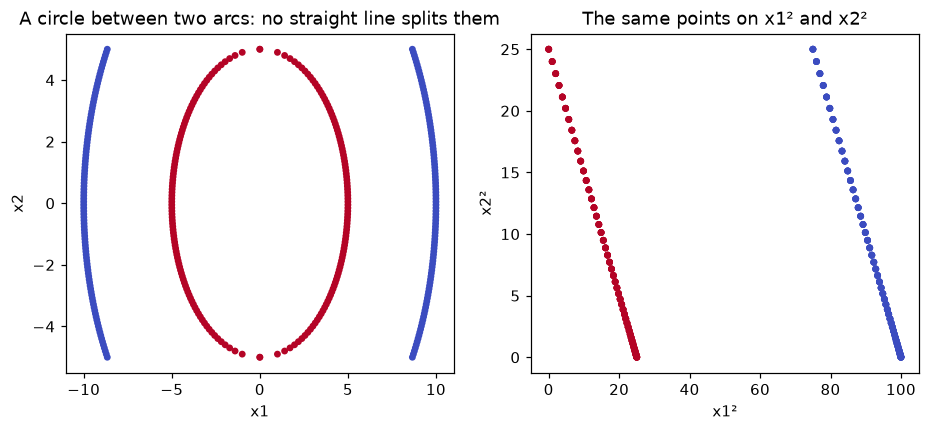
What the circles show
- A linear SVC on x₁ and x₂ scores 0.45, worse than guessing, because the arcs lie on both sides of the circle.
- On the five polynomial features the same linear SVC scores 1.0. In the right-hand plot the circle lies on the line x₁² + x₂² = 25 and the arcs on x₁² + x₂² = 100, so a straight line splits them.
- kernel="poly" with its defaults scores 0.590; with degree=2 and coef0=1, the video's formula, it scores 1.000. The rbf kernel scores 1.000 too, and the sigmoid kernel 0.510.
Choosing a kernel and its settings
On a less tidy dataset the kernels differ less, and the settings matter as much as the kernel. 1,000 points from make_classification, two features and two clusters per class, are fitted with each of the four kernels, then the rbf kernel is tuned over C and gamma.
from sklearn.datasets import make_classification
from sklearn.model_selection import train_test_split, GridSearchCV
from sklearn.svm import SVC

X, y = make_classification(n_samples=1000, n_features=2, n_classes=2, n_clusters_per_class=2,
                           n_redundant=0, random_state=1)
X_train, X_test, y_train, y_test = train_test_split(X, y, test_size=0.25, random_state=10)
for kernel in ("linear", "rbf", "poly", "sigmoid"):
    print(f"{kernel:8} test accuracy {SVC(kernel=kernel).fit(X_train, y_train).score(X_test, y_test):.3f}")

param_grid = {"C": [0.1, 1, 10, 100, 1000], "gamma": [1, 0.1, 0.01, 0.001, 0.0001], "kernel": ["rbf"]}
grid = GridSearchCV(SVC(), param_grid, cv=5).fit(X_train, y_train)
print("best:", grid.best_params_, f" test accuracy {grid.score(X_test, y_test):.3f}")linear test accuracy 0.832
rbf test accuracy 0.852
poly test accuracy 0.812
sigmoid test accuracy 0.772
best: {'C': 1, 'gamma': 1, 'kernel': 'rbf'} test accuracy 0.852What the four kernels scored
- The rbf kernel scores highest, 0.852, then linear 0.832, polynomial 0.812 and sigmoid 0.772.
- The grid picks C = 1 and gamma = 1 and scores 0.852 again: on this data the tuned settings do no better than the defaults.
Polynomial kernel vs rbf kernel
| Polynomial kernel | rbf kernel | |
|---|---|---|
| Formula | (γ·aᵀb + coef0)^degree | e^(−γ‖a − b‖²) |
| New features it stands for | every product of the features up to the degree | infinitely many; a similarity that fades with distance |
| Settings | degree, coef0, gamma, C | gamma, C |
| Good for | boundaries of a known shape, such as circles (degree 2) | a default when the shape is unknown |
| scikit-learn | SVC(kernel="poly") | SVC(kernel="rbf"), the default |
Where you use SVM kernels
- Curved class boundaries on small and medium datasets, where a linear SVM underfits.
- Image and text classification with a few thousand rows, such as handwritten digits, where an rbf SVM is a strong baseline.
- Support vector regression: Support vector regression (SVR) takes the same kernels.
kernel="poly" defaults to degree=3 and coef0=0, which drops the lower terms of the video's (aᵀb + 1)d. On the circles that kernel scored far below the degree=2, coef0=1 version. Set coef0 when you want the + 1.Related
- Previous: Support vector regression (SVR)
- Next: K-means clustering
- See also: Hyperparameter tuning with GridSearchCV
- Reference: scikit-learn user guide, Kernel functions
- Remove the
x ** 2column fromtwo_dand usenp.c_[x, np.abs(x)]instead: does a linear SVC still separate the classes? - Change
{"degree": 2, "coef0": 1}to{"degree": 2, "coef0": 0}on the circles and compare the accuracy. - Change
random_state=1torandom_state=0in make_classification and check whether the four kernels keep their order.
This is what real progress feels like.