Overfitting and underfitting
Overfitting is a modelling failure in which a model fits its training data almost perfectly but predicts new data badly; underfitting is the opposite failure, in which the model is poor on the training data and on new data alike.
Last updated: 05 Oct, 2026 · scikit-learn 1.9.1
A model is only useful on data it has not seen. Comparing its score on the training data with its score on the test data tells you whether it learned the pattern, memorised the points, or learned too little.
Fitting a line through two points
The video starts from the cost function of the Cost function lesson, J(θ₀, θ₁) = 1/2m Σ (hθ(x(i)) − y(i))², and a data set with only two points. The best fit line passes through both points and through the origin, so θ₀ = 0 and every error is zero. The cost is J = 0, the smallest value it can take.
These two points are the training data, the data the model learns from. Now new points arrive, the test data. For a new point the line predicts a value on the line, while the real value sits far below it. The gap between the predicted point and the real point is large. That condition is called overfitting.
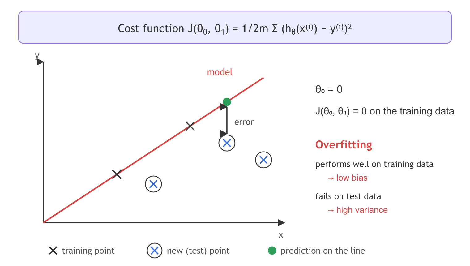
In the words of the video, an overfit model "performs well with training data but it fails to perform well with test data". Doing well on the training data is called low bias. Failing on the test data is called high variance. The Bias and variance lesson defines both terms properly.
The board labels the underfit model "high bias, high variance"; the usual reading is high bias with low variance, because its training and test scores (70% and 65%) are close together.
Comparing train and test accuracy
Underfitting is the second failure: the model accuracy is bad on the training data and also bad on the test data. The model has not learned the pattern at all. The video then puts three models side by side.
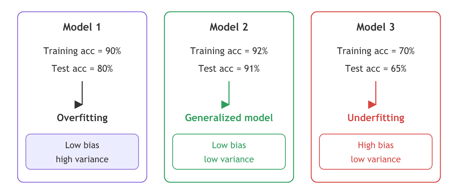
- Model 1, 90% train and 80% test. Good on the training data, a clear drop on the test data: overfitting, low bias and high variance.
- Model 2, 92% train and 91% test. Good on both, and the two scores are almost equal: a generalized model, low bias and low variance.
- Model 3, 70% train and 65% test. Poor on both: underfitting, high bias. The small gap between the scores means low variance.
The generalized model is the one you want, because when new data comes it still gives good output. Back on the two-point example, the red line has low bias and high variance: perfect on its own two points, far off on every new one.
Overfitting a polynomial on noisy data
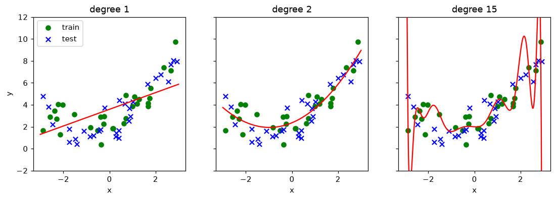
The two-point line is the smallest case. In code the same thing appears when a model has far more freedom than the data needs. Below, 60 points follow the curve y = 0.5x² + x + 2 plus random noise, and half of them are held back as test data with train_test_split (see Train and test split). Three models are fitted on the training half: a straight line (degree 1), a curve with an x² term (degree 2) and a degree 15 polynomial.
The scores are R², from the R squared and adjusted R squared lesson: 1 is a perfect fit, 0 is no better than always predicting the mean, and a value below 0 is worse than predicting the mean.
Making polynomial features
PolynomialFeatures turns the one column x into the columns 1, x, x², up to the chosen degree. LinearRegression then fits one coefficient per column, so a straight-line model can bend. StandardScaler puts the columns on one scale, which keeps the degree 15 fit numerically stable. make_pipeline chains the three steps: fit runs them in order and passes each step's output to the next.
from sklearn.pipeline import make_pipeline
from sklearn.preprocessing import PolynomialFeatures, StandardScaler
from sklearn.linear_model import LinearRegression

# degree 2: the columns 1, x and x² go into one linear regression
model = make_pipeline(PolynomialFeatures(degree=2), StandardScaler(), LinearRegression())
model.fit(X_train, y_train)
print(model.score(X_test, y_test))     # R² on the test data
Scoring degree 1, 2 and 15
The loop fits the three models on the same training points, prints both scores and draws each fitted curve over the data.
import numpy as np
import matplotlib.pyplot as plt
from sklearn.model_selection import train_test_split
from sklearn.pipeline import make_pipeline
from sklearn.preprocessing import PolynomialFeatures, StandardScaler
from sklearn.linear_model import LinearRegression

rng = np.random.RandomState(0)
X = rng.uniform(-3, 3, 60).reshape(-1, 1)
y = 0.5 * X[:, 0] ** 2 + X[:, 0] + 2 + rng.normal(0, 1, 60)
X_train, X_test, y_train, y_test = train_test_split(X, y, test_size=0.5, random_state=42)

grid = np.linspace(-3, 3, 300).reshape(-1, 1)
fig, axes = plt.subplots(1, 3, figsize=(12, 3.6), sharey=True)
for ax, degree in zip(axes, [1, 2, 15]):
    model = make_pipeline(PolynomialFeatures(degree=degree), StandardScaler(), LinearRegression())
    model.fit(X_train, y_train)
    train_r2 = model.score(X_train, y_train)
    test_r2 = model.score(X_test, y_test)
    print(f"degree {degree:2}: train R2 = {train_r2:.2f}, test R2 = {test_r2:.2f}")
    ax.scatter(X_train, y_train, color="green", label="train")
    ax.scatter(X_test, y_test, color="blue", marker="x", label="test")
    ax.plot(grid, model.predict(grid), color="red")
    ax.set_title(f"degree {degree}")
    ax.set_xlabel("x")
    ax.set_ylim(-2, 12)
axes[0].set_ylabel("y")
axes[0].legend()
plt.show()degree 1: train R2 = 0.42, test R2 = 0.45 degree 2: train R2 = 0.77, test R2 = 0.82 degree 15: train R2 = 0.88, test R2 = -2.35
What the three scores show
- Degree 1 underfits. Train R² 0.42 and test R² 0.45: both low and close together. A straight line cannot follow the bend, which is high bias with low variance, the video's model 3.
- Degree 2 generalizes. Train 0.77 and test 0.82: good on both, with no drop on new points. The model has the same shape as the curve that made the data, the video's model 2.
- Degree 15 overfits. It has the best training score, 0.88, and a test R² of −2.35, worse than predicting the mean. It bends through the training points and swings far away between them, the two-point line again.
- The training score alone misleads. It rises with every extra degree. Only the test score shows that degree 15 is the worst model of the three.
Overfitting vs underfitting
| Overfitting | Generalized model | Underfitting | |
|---|---|---|---|
| Training score | high | high | low |
| Test score | much lower than training | close to training | low, close to training |
| Bias / variance | low bias, high variance | low bias, low variance | high bias, low variance |
| Typical cause | model too flexible for the data | flexibility matches the pattern | model too simple |
| What helps | more data, a simpler model, Ridge or Lasso | keep it | more features, a more flexible model |
Where you use the train and test comparison
- After every fit. Print the training and the test score together; the gap tells you which failure you have before you tune anything.
- Choosing model complexity. The polynomial degree here, the depth of a decision tree later: raise it while the test score improves, stop when it drops.
- Choosing regularization. Ridge regression and Lasso regression exist to pull an overfit model back toward the generalized one.
Related
- Previous: Cross-validation
- Next: Bias and variance
- Reference: scikit-learn: Underfitting vs. Overfitting
- Change the degrees to
[1, 2, 5]. Degree 5 has a little more freedom than the curve needs; compare its test R² with degree 2. - Change 60 to 600 in both
rng.uniformandrng.normal. With ten times more training points, degree 15 has much less room to overfit. - Change the noise
rng.normal(0, 1, 60)torng.normal(0, 0.2, 60)and see how the three train scores move.
Every expert started right here.