XGBoost classifier
XGBoost (extreme gradient boosting) is a boosting algorithm that builds binary decision trees one after another on the residuals of the model so far, choosing each split by the gain in similarity weight.
Last updated: 05 Oct, 2026 · XGBoost 3.4.1
Gradient boosting fits each new tree to the residuals of the model so far. XGBoost follows the same plan with its own way of building each tree: a similarity weight, a gain and a penalty λ. It solves both classification and regression; this lesson is the classifier, on the same loan table as AdaBoost.
Starting from a base model and residuals
The video's dataset decides loan approval from salary and credit score. Salary is either ≤50K or >50K; credit is bad (B), good (G) or normal (N); approval is 0 or 1.
| Salary | Credit | Approval | Residual |
|---|---|---|---|
| ≤50K | B | 0 | −0.5 |
| ≤50K | G | 1 | 0.5 |
| ≤50K | G | 1 | 0.5 |
| >50K | B | 0 | −0.5 |
| >50K | G | 1 | 0.5 |
| >50K | N | 1 | 0.5 |
| ≤50K | N | 0 | −0.5 |
XGBoost first creates a base model, a weak learner that outputs a probability of 0.5 for every record whatever the input. The residual of a record is its approval minus that probability: 0 − 0.5 = −0.5 and 1 − 0.5 = 0.5. The next trees are trained on these residuals, in sequence.
Building a binary tree on the residuals
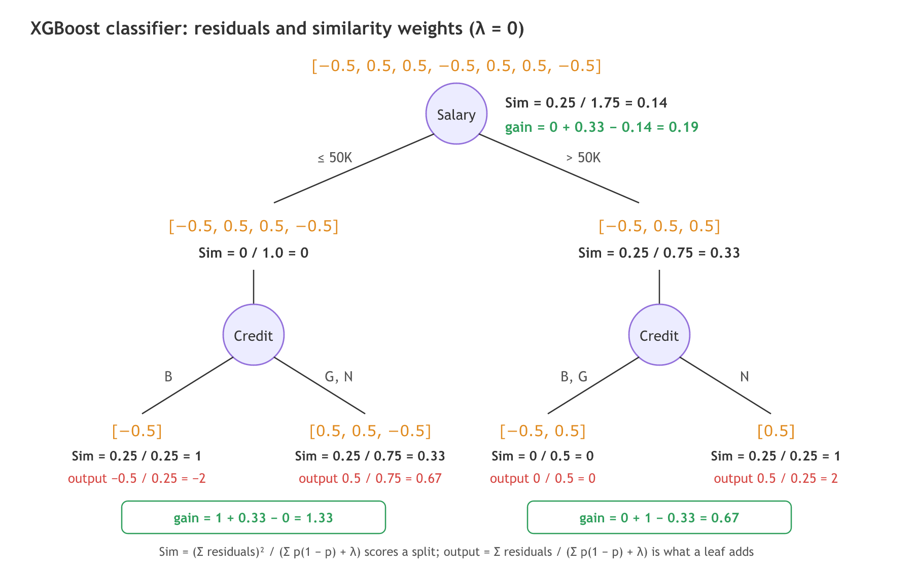
The steps are: (1) build a binary decision tree using the features, (2) calculate the similarity weight of each node, (3) calculate the gain of the split. The tree is always binary, so a feature with three categories, like credit, is split into two groups.
The video starts with salary. The root holds all seven residuals, [−0.5, 0.5, 0.5, −0.5, 0.5, 0.5, −0.5]. The ≤50K branch gets the residuals of records 1, 2, 3 and 7: [−0.5, 0.5, 0.5, −0.5]. The >50K branch gets records 4, 5 and 6: [−0.5, 0.5, 0.5].
The video once says “probability minus approval”; the board and the numbers use approval minus probability, the correct order.
Calculating the similarity weight
The similarity weight scores how alike the residuals in a node are. The residuals are added first and the sum is squared. The bottom adds p(1 − p) for every record in the node, where p is the probability from the base model, plus λ (lambda), a hyperparameter that stops the tree from overfitting. The video sets λ = 0 for the worked numbers.
The board writes the bottom as Σ(p(1 − p) + λ), which would add λ once per record; λ is added once. For the ≤50K branch the residuals cancel: (−0.5 + 0.5 + 0.5 − 0.5)² = 0, so its similarity weight is 0. For the >50K branch, (−0.5 + 0.5 + 0.5)² = 0.25 and 3 × 0.5 × 0.5 = 0.75, so it is 0.25 / 0.75 = 0.33.
Calculating the gain of the salary split
The root's residuals add up to 0.5, so its similarity weight is 0.25 / (7 × 0.25) = 0.25 / 1.75 = 0.14. The gain of a split is the similarity of the two branches minus the similarity of the node they came from.
The board calls this information gain, the same name as in Information gain, but here it is computed from similarity weights. XGBoost compares the gain of every candidate split and keeps the highest. The video assumes salary gives the highest gain so that it can show the steps; the code below checks that assumption.
Splitting the ≤50K branch on credit
The ≤50K branch is split again, on credit. Credit has three categories, so the binary split puts B on one side and G, N on the other. B gets record 1, residual [−0.5]: similarity 0.25 / 0.25 = 1. G, N gets records 2, 3 and 7, [0.5, 0.5, −0.5]: similarity 0.25 / 0.75 = 0.33. The node above has similarity 0, so the gain is 1 + 0.33 − 0 = 1.33.
The >50K branch can be split on credit too, with B and G on one side and N on the other: [−0.5, 0.5] has similarity 0 / 0.5 = 0 and [0.5] has 0.25 / 0.25 = 1, so the gain is 0 + 1 − 0.33 = 0.67. The tree now has four leaves.
Predicting a probability with the sigmoid
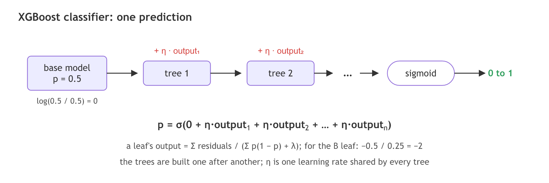
To predict record 1, it first goes to the base model. The probability 0.5 is turned into log-odds, log(p / (1 − p)) = log(0.5 / 0.5) = 0. The record then follows the tree: ≤50K, then credit B. The leaf's output is multiplied by the learning rate α and added. A sigmoid turns the total into a probability between 0 and 1. With more trees the output is σ(0 + α·tree₁ + α·tree₂ + … + α·treeₙ): each tree's output is added slowly, which is what makes it boosting.
Two points differ from the board. First, the number a leaf adds is its output value, Σ residuals / (Σ p(1 − p) + λ), not its similarity weight. For the B leaf that is −0.5 / 0.25 = −2, so record 1 gets σ(0 + α·(−2)), not σ(0 + α·1). The similarity weight only scores splits. Second, XGBoost uses one learning rate for every tree, and it builds the trees one after another, each on the residuals left by the trees before it. The video says the trees are built in parallel; XGBoost runs in parallel only inside one tree, when it searches for the best split.
XGBoost is a black box model: with hundreds of trees nobody follows the calculation by hand. It still overfits, so its trees are limited in advance (pre-pruning) with settings such as max_depth, and λ is tuned with cross-validation.
Computing the board's similarity weights and gains
The table typed in, a function for the similarity weight, and the two splits from the board. The last line scores credit at the root, the split the video does not try.
The similarity weight as a function
p = 0.5                                    # the base model's probability for every record
res = approval - p                         # residual = approval - probability

def sim(r, lam=0.0):
    # (sum of residuals) squared, over the sum of p(1 - p) plus lambda
return r.sum() ** 2 / (len(r) * p * (1 - p) + lam)import numpy as np
approval = np.array([0, 1, 1, 0, 1, 1, 0])
salary = np.array(["<=50K", "<=50K", "<=50K", ">50K", ">50K", ">50K", "<=50K"])
credit = np.array(["B", "G", "G", "B", "G", "N", "N"])
p = 0.5
res = approval - p
def sim(r, lam=0.0):
return r.sum() ** 2 / (len(r) * p * (1 - p) + lam)
root = sim(res)
left, right = res[salary == "<=50K"], res[salary == ">50K"]
print("residuals:", res)
print(f"root {root:.2f} <=50K {sim(left):.2f} >50K {sim(right):.2f}")
print(f"gain of the salary split: {sim(left) + sim(right) - root:.2f}")
cl = credit[salary == "<=50K"]
b, gn = left[cl == "B"], left[cl != "B"]
print(f"under <=50K: B {sim(b):.2f} G,N {sim(gn):.2f} gain {sim(b) + sim(gn) - sim(left):.2f}")
print(f"leaf output of B: {b.sum() / (len(b) * p * (1 - p)):.1f}")
cr = credit[salary == ">50K"]
bg, n = right[cr != "N"], right[cr == "N"]
print(f"under >50K: B,G {sim(bg):.2f} N {sim(n):.2f} gain {sim(bg) + sim(n) - sim(right):.2f}")
b_all, gn_all = res[credit == "B"], res[credit != "B"]
print(f"credit B vs G,N at the root: gain {sim(b_all) + sim(gn_all) - root:.2f}")residuals: [-0.5 0.5 0.5 -0.5 0.5 0.5 -0.5] root 0.14 <=50K 0.00 >50K 0.33 gain of the salary split: 0.19 under <=50K: B 1.00 G,N 0.33 gain 1.33 leaf output of B: -2.0 under >50K: B,G 0.00 N 1.00 gain 0.67 credit B vs G,N at the root: gain 3.66
What the similarity weights and gains show
- The board's numbers come out exactly: root 0.14, ≤50K 0, >50K 0.33, gain 0.19; under ≤50K, B 1, G,N 0.33, gain 1.33.
- The split of the >50K branch gives B,G 0 and N 1, for a gain of 0.67.
- The B leaf's output is −2.0, the number a prediction uses, while its similarity weight is 1.
- Credit at the root has a gain of 3.66, far above salary's 0.19. A real XGBoost run would start with credit, which is what the library does below.
Computing the second-round residuals
The first tree changes every record's probability, and the second tree trains on what is left. With a learning rate of 0.1, record 1 (≤50K, B) lands in the leaf with output −2. Its log-odds become 0 + 0.1 × (−2) = −0.2, its probability σ(−0.2) = 0.450, and its new residual 0 − 0.450 = −0.450, a little closer to 0 than −0.5. Record 2 (≤50K, G) lands in the leaf with output 0.67: 0 + 0.1 × 0.67 = 0.067, probability 0.517, residual 1 − 0.517 = 0.483.
| # | Salary | Credit | Approval | R1 | Leaf output | p after tree 1 | R2 |
|---|---|---|---|---|---|---|---|
| 1 | ≤50K | B | 0 | −0.5 | −2 | 0.450 | −0.450 |
| 2 | ≤50K | G | 1 | 0.5 | 0.67 | 0.517 | 0.483 |
| 3 | ≤50K | G | 1 | 0.5 | 0.67 | 0.517 | 0.483 |
| 4 | >50K | B | 0 | −0.5 | 0 | 0.500 | −0.500 |
| 5 | >50K | G | 1 | 0.5 | 0 | 0.500 | 0.500 |
| 6 | >50K | N | 1 | 0.5 | 2 | 0.550 | 0.450 |
| 7 | ≤50K | N | 0 | −0.5 | 0.67 | 0.517 | −0.517 |
Records 4 and 5 keep their residuals, because their leaf outputs 0; record 7 moves away from its label, because it shares a leaf with records 2 and 3. The second tree uses the same formulas, but p(1 − p) is no longer 0.25 for everyone: for record 1 it is 0.450 × 0.550 = 0.248.
The second-round residuals as code
leaves = [(salary == "<=50K") & (credit == "B"), (salary == "<=50K") & (credit != "B"),
          (salary == ">50K") & (credit != "N"), (salary == ">50K") & (credit == "N")]
log_odds = np.zeros(7)                           # the base model: log(0.5 / 0.5) = 0
for leaf in leaves:
    output = res[leaf].sum() / (leaf.sum() * p * (1 - p))     # the leaf output, lambda = 0
    log_odds[leaf] += 0.1 * output                             # learning rate 0.1
p1 = 1 / (1 + np.exp(-log_odds))                 # the sigmoid
res2 = approval - p1 # the residuals tree 2 trains onleaves = [(salary == "<=50K") & (credit == "B"), (salary == "<=50K") & (credit != "B"),
(salary == ">50K") & (credit != "N"), (salary == ">50K") & (credit == "N")]
log_odds = np.zeros(7)
for leaf in leaves:
output = res[leaf].sum() / (leaf.sum() * p * (1 - p))
log_odds[leaf] += 0.1 * output
p1 = 1 / (1 + np.exp(-log_odds))
res2 = approval - p1
print("log-odds after tree 1: ", log_odds.round(3))
print("probabilities: ", p1.round(3))
print("second-round residuals: ", res2.round(3))
print("p(1 - p) for tree 2: ", (p1 * (1 - p1)).round(3))log-odds after tree 1: [-0.2 0.067 0.067 0. 0. 0.2 0.067] probabilities: [0.45 0.517 0.517 0.5 0.5 0.55 0.517] second-round residuals: [-0.45 0.483 0.483 -0.5 0.5 0.45 -0.517] p(1 - p) for tree 2: [0.248 0.25 0.25 0.25 0.25 0.248 0.25 ]
What the second round starts from
- The log-odds after tree 1 are 0.1 times the leaf output: −0.2, 0.067, 0 and 0.2.
- The probabilities are 0.45, 0.517, 0.5 and 0.55, and the second-round residuals −0.45, 0.483, −0.5, 0.5, 0.45 and −0.517, as in the table above.
- p(1 − p) is 0.248 for records 1 and 6 and 0.25 for the rest; it goes into the bottom of the second tree's similarity weights.
Fitting XGBClassifier on the loan table
The XGBoost library's scikit-learn style classes are XGBClassifier and XGBRegressor. It installs with pip install xgboost==3.4.1; on macOS it also needs brew install libomp, as Installing scikit-learn explains.
Matching the board's settings
Each setting maps to a part of the board. base_score=0.5 is the base model. reg_lambda=0 is λ = 0. learning_rate is the α the video multiplies by. min_child_weight=0 lets a leaf hold one record, because one record's p(1 − p) is 0.25, below the default minimum of 1. tree_method="exact" tries every split value.
from xgboost import XGBClassifier

model = XGBClassifier(n_estimators=1, max_depth=2, learning_rate=0.3, reg_lambda=0,
                      min_child_weight=0, base_score=0.5, tree_method="exact")
Printing the tree with its gains
get_booster().get_dump(with_stats=True) prints each tree as text: the split, its gain, and each leaf's value. cover is the node's Σ p(1 − p). The printed leaf value already includes the learning rate.
import pandas as pd
from xgboost import XGBClassifier

X = pd.DataFrame({"salary_over_50k": (salary == ">50K").astype(int),
                  "credit_bad": (credit == "B").astype(int)})
model = XGBClassifier(n_estimators=1, max_depth=2, learning_rate=0.3, reg_lambda=0,
                      min_child_weight=0, base_score=0.5, tree_method="exact")
model.fit(X, approval)
print(model.get_booster().get_dump(with_stats=True)[0])

p1 = model.predict_proba(X.iloc[[0]])[0, 1]
print("record 1, probability of approval:", round(float(p1), 4))
print("by hand, sigmoid(0 + 0.3 * -2): ", round(1 / (1 + np.exp(0.6)), 4))0:[credit_bad<1] yes=1,no=2,missing=1,gain=3.65714312,cover=1.75 1:[salary_over_50k<1] yes=3,no=4,missing=3,gain=0.533333182,cover=1.25 3:leaf=0.200000018,cover=0.75 4:leaf=0.600000024,cover=0.5 2:leaf=-0.600000024,cover=0.5 record 1, probability of approval: 0.3543 by hand, sigmoid(0 + 0.3 * -2): 0.3543
What the fitted tree says
- The root splits on credit_bad with gain 3.657, the 3.66 computed by hand, and cover 1.75 = 7 × 0.25.
- The credit-bad leaf is −0.6: the output −2 times the learning rate 0.3.
- Under good and normal credit the tree splits on salary (gain 0.533), the other order of the video's two splits.
- Record 1's probability is 0.3543 both from the library and from σ(0 + 0.3 × (−2)) by hand, so the leaf output, not the similarity weight, is what goes into the prediction.
Classifying tumours with 200 trees
On a real dataset XGBoost runs with many trees and the defaults for the base score. The breast cancer split is the same as in Random forest, so the two scores compare.
clf = XGBClassifier(n_estimators=200, max_depth=3, learning_rate=0.1, reg_lambda=1,
                    random_state=0)
clf.fit(X_train, y_train)from sklearn.datasets import load_breast_cancer
from sklearn.model_selection import train_test_split
from xgboost import XGBClassifier
X, y = load_breast_cancer(return_X_y=True)
X_train, X_test, y_train, y_test = train_test_split(X, y, test_size=0.3, random_state=0)
clf = XGBClassifier(n_estimators=200, max_depth=3, learning_rate=0.1, reg_lambda=1,
random_state=0)
clf.fit(X_train, y_train)
print(f"test accuracy: {clf.score(X_test, y_test):.3f}")
print("probabilities of benign, first 3 test tumours:", clf.predict_proba(X_test[:3])[:, 1].round(3))test accuracy: 0.965 probabilities of benign, first 3 test tumours: [0.001 0.982 0.999]
Reading the tumour results
- Test accuracy 0.965, a little above the random forest's 0.959 on the same split.
- The probabilities are the sigmoid outputs of 200 trees added together; a value above 0.5 is predicted benign.
XGBoost vs gradient boosting
| XGBoost | Gradient boosting in scikit-learn | |
|---|---|---|
| Each new tree learns | the residuals of the model so far | the residuals of the model so far |
| How a split is chosen | gain in similarity weight, which uses Σ p(1 − p) and λ | how much the split lowers the squared error of the residuals (criterion "friedman_mse") |
| Penalties inside the tree | reg_lambda (λ), gamma (a minimum gain), min_child_weight | max_depth, min_samples_leaf |
| Base model | base_score: 0.5 in the video, estimated from the labels when unset | the log-odds of the class share (classifier), the mean (regressor) |
| Where it lives | the xgboost package: XGBClassifier, XGBRegressor | sklearn.ensemble: GradientBoostingClassifier, GradientBoostingRegressor |
Where you use the XGBoost classifier
- Credit and loan approval on tabular data, like the video's salary and credit example.
- Fraud and churn prediction, where many weak signals across columns add up.
- Kaggle-style tabular problems, where gradient boosted trees are the usual strong baseline.
base_score is not set, XGBoost 3.4.1 estimates it from the labels instead of starting at 0.5: on the loan table it starts from 0.571, the share of approvals. Pass base_score=0.5 when you want the video's base model and the board's residuals.Related
- Previous: Gradient boosting
- Next: XGBoost regressor
- See also: Logistic regression for the sigmoid and log-odds
- Reference: Introduction to boosted trees in the XGBoost docs
- Call
sim(left, lam=1)andsim(right, lam=1)to see how λ = 1 shrinks the similarity weights. - Set
learning_rate=1.0in the one-tree model and check that the credit-bad leaf prints −2. - Remove
min_child_weight=0and print the dump again: every split would leave a leaf with a cover below 1, so the tree is a single leaf.
Every expert started right here.