Curse of dimensionality
The curse of dimensionality is a problem in machine learning that makes a model worse as it is given more and more features, many of which carry little or no information about the output.
Last updated: 05 Oct, 2026 · scikit-learn 1.9.1
The clustering lessons up to DBSCAN used two features, so every group could be drawn. Real datasets often have hundreds. This lesson shows what too many features do to a model, and the first of the two fixes, feature selection; the second fix is Principal component analysis (PCA).
Adding features until the accuracy falls
A dimension is a feature. The video's dataset predicts the price of a house from 500 features, such as house size, number of bedrooms and number of bathrooms. Six models get more and more of them: M1 the three most important, M2 six, M3 fifteen, M4 fifty, M5 a hundred, and M6 all 500.
While the new features matter, accuracy rises: accuracy 2 beats accuracy 1, and accuracy 3 beats accuracy 2. From M4 on, many of the added features have little or no importance, but the model still learns from them. Accuracy 4 falls below accuracy 3, and accuracy 5 and 6 fall further. That fall is the curse of dimensionality.
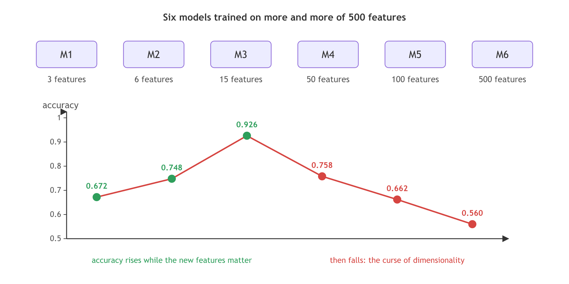
The accuracies on the diagram come from the run further down, which trains the six models on generated data where only 15 of the 500 features carry information.
Slowing down and confusing the model
The video's second point is time. Every feature is one more dimension in the model's equations, so the more features there are, the more calculation each training step needs, and the model performance degrades in that sense too.
Then comes an example. Ask a person who knows the market what a house costs in location A. With one feature, the location, the guess is 450k to 500k. Asked for a 3BHK apartment, the person moves the guess to 500k to 600k. Near a beach, the price rises; near a celebrity's house, it rises again. Grocery shops nearby add a little, and then comes the number of schools around. With every request the person has more to weigh, gets confused, and the answer gets less accurate. A model fed many features is confused in the same way: the video calls it overfed.
Reasons to reduce the dimensions
The board notes list three reasons for dimensionality reduction, a common interview question:
- Prevent the curse of dimensionality, the fall in accuracy above.
- Improve the performance of the model: fewer dimensions means less calculation and faster training.
- Visualise the data: people can see at most three dimensions, so 100 features reduced to 2 or 3 can be plotted and understood.
There are two ways out. Feature selection keeps the most important of the original features and drops the rest. Feature extraction, the idea behind dimensionality reduction, derives a few new features from all of them, as PCA does in the next lesson. This lesson does feature selection.
Measuring a relationship with covariance and Pearson correlation
Feature selection needs a number for how an input x and the output y move together. Covariance is that number, divided by n − 1 because the data is a sample:
A positive covariance means y rises when x rises and falls when x falls: a positive linear relationship. A negative covariance means y falls as x rises, an inverse linear relationship. A value near 0 means no relationship: the scatter plot is a round cloud. A feature with a strong covariance with the output is an important feature; one near 0 can be removed. Covariance has no fixed range, though: it can be any positive or negative number. Pearson correlation divides it by the two standard deviations, which keeps it between −1 and +1:
The clip reads this formula as covariance multiplied by the two standard deviations; the board notes divide, and dividing is what keeps r between −1 and +1. The nearer r is to +1, the more positively correlated x and y are; the nearer to −1, the more negatively correlated; near 0 there is no linear relationship.
Dropping fountain size from the housing data
The video's housing data has two input features, house size and fountain size, and the output, the price. Plotted against price, house size shows a clear linear relationship, so it is an important feature. Fountain size shows none: the price stays in the same band whatever the size of the fountain, with a correlation near 0, somewhere between 0 and 0.25. So fountain size is dropped. That is feature selection with covariance and correlation.
Covariance and correlation by hand
x, y = df["house_size"], df["price"]
cov = ((x - x.mean()) * (y - y.mean())).sum() / (len(df) - 1)   # the formula above
r = cov / (x.std() * y.std())                                    # Pearson correlation
Every pair at once with cov and corr
print(df.cov())    # covariance of every pair of columns, divided by n - 1
print(df.corr())   # Pearson correlation of every pair, from -1 to +1
Computing covariance and correlation for eight houses
Eight made-up houses, with prices that rise with the house size and fountain sizes that follow no pattern:
import pandas as pd

# Eight houses: size in square feet, fountain size in square feet, price in $1000s
df = pd.DataFrame({
    "house_size":    [800, 950, 1100, 1200, 1400, 1550, 1700, 1900],
    "fountain_size": [12, 30, 8, 25, 15, 10, 28, 18],
    "price":         [400, 460, 520, 570, 660, 710, 800, 880],
})

x, y = df["house_size"], df["price"]
cov = ((x - x.mean()) * (y - y.mean())).sum() / (len(df) - 1)
r = cov / (x.std() * y.std())
print("Cov(house_size, price) by hand:", round(cov, 1), " pandas:", round(df.cov().loc["house_size", "price"], 1))
print("Pearson r by hand:", round(r, 3))
print(df.corr().round(3)["price"])Cov(house_size, price) by hand: 63500.0 pandas: 63500.0 Pearson r by hand: 0.999 house_size 0.999 fountain_size 0.101 price 1.000 Name: price, dtype: float64
What the two correlations say
- The hand formula and pandas agree on the covariance of house size and price.
- House size has r = 0.999 with price, almost a straight line: keep it.
- Fountain size has r = 0.101 with price, inside the video's 0 to 0.25: drop it.
- Covariance alone could not say this: its value is in square feet times thousands of dollars, so its size means little until it is divided by the standard deviations.
Training six models on more and more features
The six models from the board can be run. make_classification builds 500 rows with 500 features, of which only 15 carry information; with shuffle=False those 15 come first, like the most important features the video gives M1 to M3. Each model is a K nearest neighbours classifier in a pipeline with StandardScaler, scored with 5-fold cross-validation on the first 3, 6, 15, 50, 100 and 500 features.
from sklearn.datasets import make_classification
from sklearn.model_selection import cross_val_score
from sklearn.neighbors import KNeighborsClassifier
from sklearn.pipeline import make_pipeline
from sklearn.preprocessing import StandardScaler

X, y = make_classification(n_samples=500, n_features=500, n_informative=15, n_redundant=0,
                           shuffle=False, random_state=1)   # the 15 useful features come first

for m, k in enumerate([3, 6, 15, 50, 100, 500], start=1):
    model = make_pipeline(StandardScaler(), KNeighborsClassifier())
    accuracy = cross_val_score(model, X[:, :k], y, cv=5).mean()
print(f"M{m}: {k:>3} features, accuracy {accuracy:.3f}")M1: 3 features, accuracy 0.672 M2: 6 features, accuracy 0.748 M3: 15 features, accuracy 0.926 M4: 50 features, accuracy 0.758 M5: 100 features, accuracy 0.662 M6: 500 features, accuracy 0.560
Why the accuracy peaks at 15 features
- M1 to M3 climb from 0.672 to 0.926: each new feature carries information.
- M4 to M6 fall to 0.758, 0.662 and 0.560: the extra features are noise, and KNN measures distances across all of them, so the noise drowns the useful ones.
- M6 with all 500 features is close to 0.5, a coin toss between the two classes. More data columns made the model worse.
Covariance vs Pearson correlation
| Covariance | Pearson correlation | |
|---|---|---|
| Range | any positive or negative number | −1 to +1 |
| Units | changes with the units of x and y | none: the same in feet or metres |
| What it tells you | the direction of the relationship | the direction and how strong it is |
| In pandas | df.cov() | df.corr() |
Where you use feature selection
- Before training: drop columns whose correlation with the output is near 0, like fountain size.
- Exploring a new dataset: a correlation table of every column against the target shows which features to look at first.
- When the features all matter, selection cannot help, and feature extraction takes over: Principal component analysis (PCA) turns room size and number of rooms into one new feature instead of dropping either.
Related
- Previous: DBSCAN
- Next: Principal component analysis (PCA)
- Reference: pandas reference: DataFrame.corr
- In the eight-house example, change fountain_size to [5, 8, 10, 14, 18, 20, 25, 30] so it rises with the price, and read its new correlation.
- In the six-model example, change n_informative=15 to n_informative=5 and see at which model the accuracy now peaks.
- Run np.corrcoef(x, x ** 2) for x = np.arange(-3, 4) and check that it prints 0 for the pair, as the Watch out says.
This is what real progress feels like.