Principal component analysis (PCA)
Principal component analysis (PCA) is a dimensionality reduction technique that turns many correlated features into a few new features, the principal components, that keep as much of the variance as possible.
Last updated: 05 Oct, 2026 · scikit-learn 1.9.1
Curse of dimensionality showed how too many features make a model worse and slower, and how feature selection drops the unimportant ones. When every feature matters, nothing can be dropped. PCA extracts two or three new features from all of the old ones instead; the breast cancer data, with 30 features, goes down to two.
Projecting onto the axis with the most spread
The video's housing example has two features, the size of the house and the number of rooms, and both drive the price. Bigger houses have more rooms, so the points rise together. The task is to turn these two dimensions into one.
The plain way is to project every point onto the size axis. The spread of the points along size is kept, and spread is what variance measures: the wider the spread, the higher the variance. The spread in the number of rooms is thrown away, so information about rooms is lost.
Finding new axes: PC1 and PC2
PCA instead transforms the axes. A new axis, size′, runs along the cloud of points, and a second one, rooms′, stands at a right angle to it. Projected onto size′, the points keep most of their spread; little is left along rooms′, so dropping it loses little.
The new axes are the principal components. PC1 captures the largest variance, PC2 the next largest, and with three features PC3 the rest. To go from 3D to 2D, keep PC1 and PC2; to go to 1D, keep PC1.
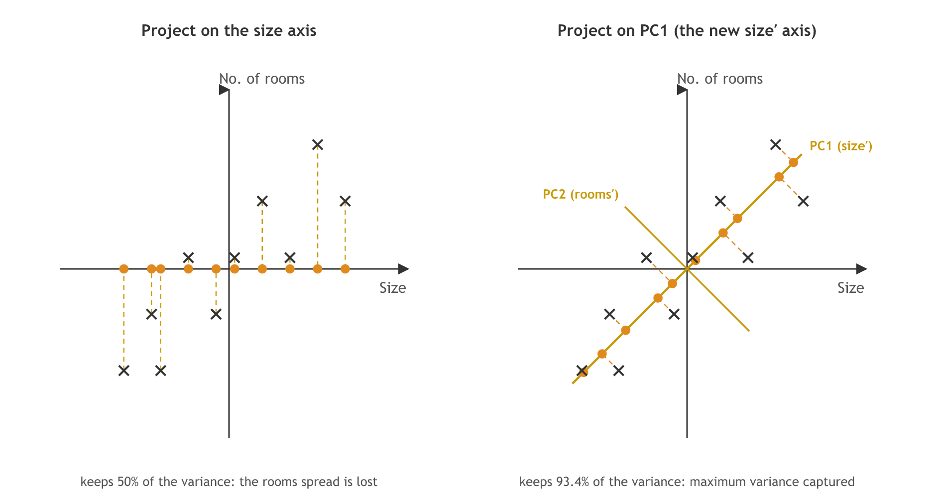
The diagram uses ten made-up houses, sizes 600 to 1800 square feet with 1 to 5 rooms, standardised. Projected onto the size axis they keep 50% of the total variance; projected onto PC1 they keep 93.4%.
The board notes call this variance the cost function. Every unit vector u gives one set of projected numbers p′₁ to p′ₙ and one variance; the goal is the unit vector with the largest one.
Eigenvectors of the covariance matrix
Trying every possible line would never end, so PCA solves for the best one. The video's steps:
- Standardise the data, so every feature has mean 0 and standard deviation 1.
- Compute the covariance matrix of the features: variances on the diagonal, covariances off it.
- Find its eigenvectors and eigenvalues, the solutions of A v = λ v.
- The eigenvector with the largest eigenvalue is PC1, the next is PC2, and so on.
The video describes the eigenvalue as the magnitude of the eigenvector. The eigenvectors here have length 1; the eigenvalue λ is the variance of the data along that eigenvector, which is why the largest λ marks PC1. The share of the variance a component keeps is its eigenvalue divided by the sum of all of them.
Computing PC1 for the house data with NumPy
import numpy as np
from sklearn.decomposition import PCA

# Ten houses: size in square feet and number of rooms
size = np.array([600, 750, 800, 950, 1100, 1200, 1350, 1500, 1650, 1800])
rooms = np.array([1, 2, 1, 3, 2, 3, 4, 3, 5, 4])
X = np.column_stack([size, rooms])

Xs = (X - X.mean(axis=0)) / X.std(axis=0)      # step 1: standardise
cov = np.cov(Xs, rowvar=False)                  # step 2: covariance matrix
values, vectors = np.linalg.eigh(cov)           # step 3: eigenvalues and eigenvectors
order = np.argsort(values)[::-1]                # largest eigenvalue first
values, vectors = values[order], vectors[:, order]
print("covariance matrix:\n", cov.round(3))
print("eigenvalues:", values.round(3))
print("PC1 direction:", vectors[:, 0].round(3))

print("variance kept on the size axis:", round(Xs[:, 0].var(ddof=1) / values.sum(), 3))
print("variance kept on PC1          :", round((Xs @ vectors[:, 0]).var(ddof=1) / values.sum(), 3))

pca = PCA(n_components=2).fit(Xs)
print("PCA explained_variance_:", pca.explained_variance_.round(3))covariance matrix: [[1.111 0.964] [0.964 1.111]] eigenvalues: [2.075 0.148] PC1 direction: [0.707 0.707] variance kept on the size axis: 0.5 variance kept on PC1 : 0.934 PCA explained_variance_: [2.075 0.148]
- The covariance matrix has 1.111 on the diagonal (standardised features, divided by n − 1) and 0.964 off it: size and rooms rise together.
- The eigenvalues are 2.075 and 0.148, and PCA's explained_variance_ prints the same two numbers.
- PC1 points along [0.707, 0.707], the diagonal of the cloud, and keeps 93.4% of the variance against 50% for the size axis.
Reducing the breast cancer data to two components
The practical loads the breast cancer data (569 rows, 30 features) into a DataFrame, standardises it with StandardScaler, then extracts two components with PCA(n_components=2). The video stresses that PCA needs the scaling step.
Standardising the 30 features
from sklearn.preprocessing import StandardScaler

scaler = StandardScaler()
scaler.fit(df)                          # mean and standard deviation per feature
scaled_data = scaler.transform(df)      # every feature now has mean 0, std 1
Fitting PCA with n_components=2
from sklearn.decomposition import PCA

pca = PCA(n_components=2)                  # keep PC1 and PC2
data_pca = pca.fit_transform(scaled_data)  # 569 rows, 2 columns
print(pca.explained_variance_) # variance along PC1 and PC2import numpy as np
import pandas as pd
from sklearn.datasets import load_breast_cancer
from sklearn.preprocessing import StandardScaler
from sklearn.decomposition import PCA
cancer_dataset = load_breast_cancer()
df = pd.DataFrame(cancer_dataset["data"], columns=cancer_dataset["feature_names"])
scaler = StandardScaler()
scaler.fit(df)
scaled_data = scaler.transform(df)
pca = PCA(n_components=2)
data_pca = pca.fit_transform(scaled_data)
print(df.shape, "->", data_pca.shape)
print(data_pca[:3].round(3))
print("explained_variance_:", pca.explained_variance_.round(3))
print("explained_variance_ratio_:", pca.explained_variance_ratio_.round(3))
# The same two numbers from the eigenvalues of the covariance matrix
eigenvalues = np.linalg.eigvalsh(np.cov(scaled_data, rowvar=False))[::-1]
print("top two eigenvalues:", eigenvalues[:2].round(3))(569, 30) -> (569, 2) [[ 9.193 1.949] [ 2.388 -3.768] [ 5.734 -1.075]] explained_variance_: [13.305 5.701] explained_variance_ratio_: [0.443 0.19 ] top two eigenvalues: [13.305 5.701]
- The first rows match the video's notebook: 9.193 and 1.949, then 2.388 and −3.768, then 5.734 and −1.075.
- explained_variance_ is [13.305, 5.701], the same as the video, and equals the top two eigenvalues of the covariance matrix.
- explained_variance_ratio_ is [0.443, 0.19]: two components keep 63.2% of the variance of 30 features.
How much variance each component keeps
The video says the variances of all the components add up to near 200 and calls the data 11 to 12 features. The breast cancer data has 30 features, and after standardising, the 30 variances add up to 30.05: each standardised feature contributes a variance of about 1. The video prints explained_variance_; explained_variance_ratio_ turns the same numbers into shares.
full = PCA()                         # no n_components: keep all 30
full.fit(scaled_data)
print("components:", full.n_components_)
print("sum of explained_variance_:", round(full.explained_variance_.sum(), 2))
print("first five ratios:", full.explained_variance_ratio_[:5].round(3))
kept = np.cumsum(full.explained_variance_ratio_)
for k in [2, 3, 6, 10]:
print(f"variance kept by {k:>2} components: {kept[k - 1]:.3f}")components: 30 sum of explained_variance_: 30.05 first five ratios: [0.443 0.19 0.094 0.066 0.055] variance kept by 2 components: 0.632 variance kept by 3 components: 0.726 variance kept by 6 components: 0.888 variance kept by 10 components: 0.952
Plotting the two components
import matplotlib.pyplot as plt

plt.figure(figsize=(8, 6))
plt.scatter(data_pca[:, 0], data_pca[:, 1], c=cancer_dataset["target"], cmap="plasma")
plt.xlabel("First principal component")
plt.ylabel("Second Principal Component")
plt.title("Breast cancer data after PCA (0 = malignant, 1 = benign)")
plt.show()
print("malignant:", (cancer_dataset["target"] == 0).sum(), " benign:", (cancer_dataset["target"] == 1).sum())malignant: 212 benign: 357
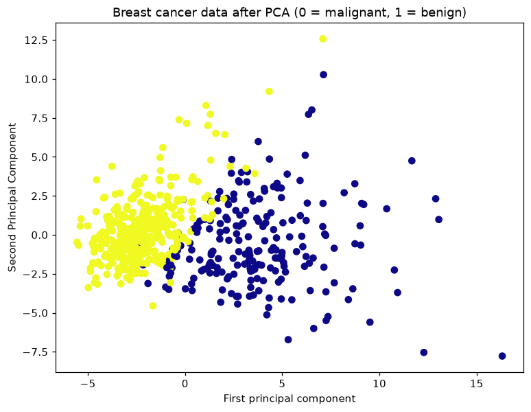
What the two components show
- Two components keep 63.2% of the variance; three keep 72.6%, six keep 88.8% and ten keep 95.2%.
- The 212 malignant and 357 benign tumours fall mostly on opposite sides of PC1, so two extracted features already separate the classes well.
- PC1 is not one of the 30 features: it is a weighted mix of all of them.
Feature extraction vs feature selection
| Feature extraction (PCA) | Feature selection | |
|---|---|---|
| What it keeps | new features built from all the old ones | a subset of the original features |
| Example from the video | size and rooms become one new feature | fountain size dropped, house size kept |
| Information lost | only the smallest variances | everything in the dropped features |
| Readable features | no: each component mixes all features | yes: the names stay |
Where you use PCA
- Plotting data with many features in 2D or 3D, as with the breast cancer plot.
- Faster training: train on 10 components that keep 95% of the variance instead of 30 features.
- Before clustering: K-means and DBSCAN measure distances, which work better on a few uncorrelated components than on many correlated features.
Related
- Previous: Curse of dimensionality
- Next: Machine learning workflow
- Reference: scikit-learn user guide: PCA
- Change PCA(n_components=2) to PCA(n_components=3) in the breast cancer example and read the three explained_variance_ratio_ values.
- Pass PCA(n_components=0.95) instead and print pca.n_components_ to see how many components keep 95%.
- Remove the StandardScaler step and fit PCA on df directly: compare explained_variance_ratio_.
Every expert started right here.