ElasticNet regression
ElasticNet regression is a linear regression that adds both the Ridge penalty, λ₁ times the squared slopes, and the Lasso penalty, λ₂ times the absolute slopes, to the cost function, so one model reduces overfitting and selects features.
Last updated: 05 Oct, 2026 · scikit-learn 1.9.1
Ridge regression shrinks every slope and Lasso regression drops some of them to 0. ElasticNet puts both penalty terms into one cost, which helps when there are many features and several of them carry the same information.
Adding both penalties to the cost function
The cost starts from the squared error of linear regression and adds two terms. The first, λ₁ Σ (slope)², is the Ridge term: it reduces overfitting. The second, λ₂ Σ |slope|, is the Lasso term: it performs feature selection. Each has its own λ, and both are hyperparameters.
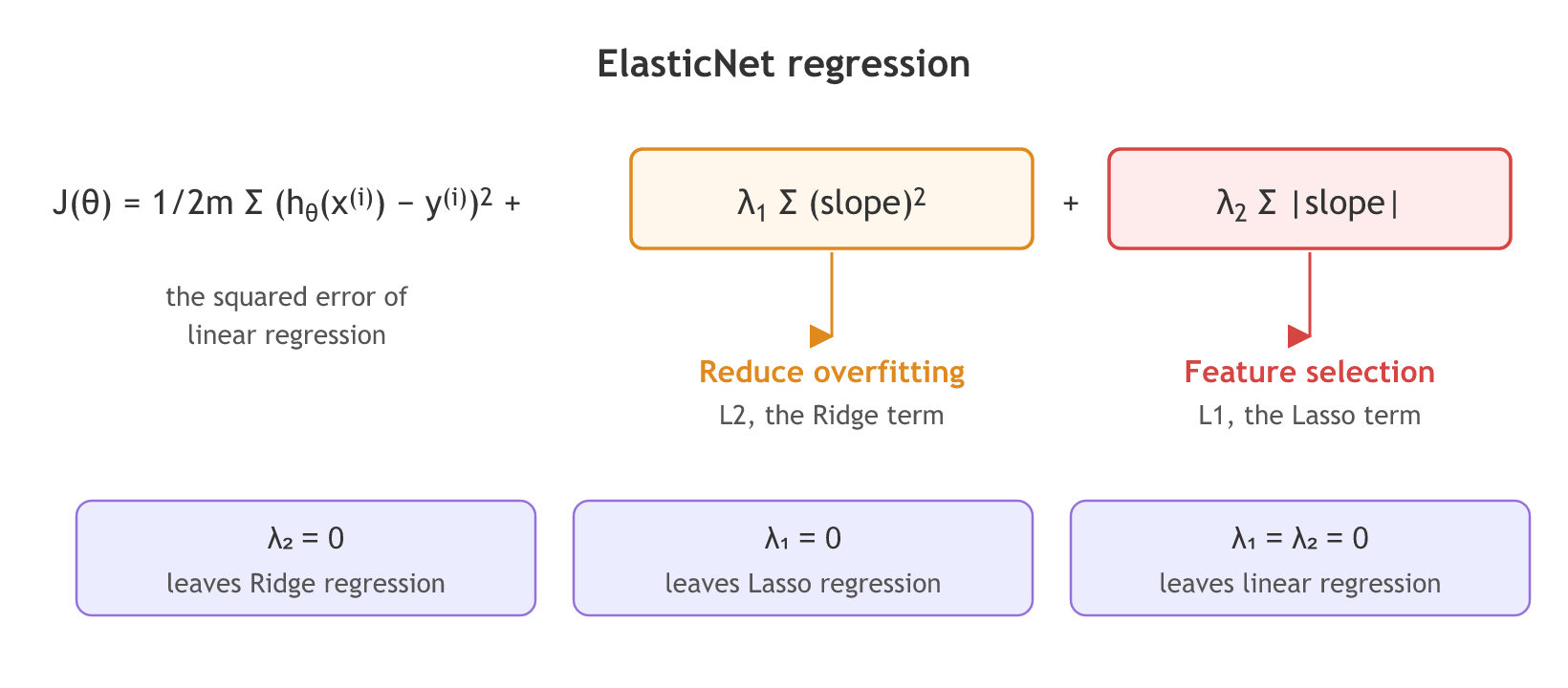
Setting λ₂ = 0 leaves Ridge, setting λ₁ = 0 leaves Lasso, and with both at 0 it is plain linear regression.
Writing the penalties with alpha and l1_ratio
scikit-learn's ElasticNet does not take λ₁ and λ₂. It takes one overall strength, alpha, and the share of it that goes to the L1 part, l1_ratio (written ρ below), a number from 0 to 1. It minimises:
Read against the cost above: λ₂ = alpha × l1_ratio and λ₁ = alpha × (1 − l1_ratio) / 2, with the squared error averaged over the n rows as in Lasso. In scikit-learn 1.9.1 the defaults are alpha = 1 and l1_ratio = 0.5, which gives λ₂ = 0.5 and λ₁ = 0.25. l1_ratio = 1 is Lasso; l1_ratio = 0 leaves only the L2 penalty.
The ElasticNet class
from sklearn.linear_model import ElasticNet

# alpha = overall strength, l1_ratio = share of the L1 (Lasso) part
elastic = ElasticNet(alpha=1.0, l1_ratio=0.5)
elastic.fit(X_train_scaled, y_train)
print(elastic.coef_)        # some slopes shrink, some are exactly 0
Comparing four models on the Algerian forest fires data
The Algerian forest fires data set has 243 days from June to September 2012 in two regions of Algeria: the weather (Temperature, relative humidity RH, wind speed Ws, Rain), the components of the fire weather index system (FFMC, DMC, DC, ISI, BUI), whether there was a fire (Classes) and the Region. The target is FWI, the Fire Weather Index. The cleaned CSV loads straight from the materials repository.
Loading the data and encoding Classes
import numpy as np
import pandas as pd
from sklearn.model_selection import train_test_split

url = "https://raw.githubusercontent.com/krishnaik06/The-Grand-Complete-Data-Science-Materials/main/Machine%20Learning/3-%20Ridge%20Lasso%20And%20Elasticnet/Ridge%20Lassso%20Elastic%20Regression%20Practicals/Algerian_forest_fires_cleaned_dataset.csv"
df = pd.read_csv(url).drop(["day", "month", "year"], axis=1)
df["Classes"] = np.where(df["Classes"].str.contains("not fire"), 0, 1)   # 1 = fire, 0 = not fire
X = df.drop("FWI", axis=1)            # 11 independent features
y = df["FWI"]                         # the Fire Weather Index
X_train, X_test, y_train, y_test = train_test_split(X, y, test_size=0.25, random_state=42)
Dropping features correlated above 0.85
Several of the index columns are computed from each other, the multicollinearity of Linear regression assumptions. The function finds every feature whose correlation with an earlier feature is above 0.85, measured on the training part only, and both parts drop it.
def correlation(dataset, threshold):
    col_corr = set()
    corr_matrix = dataset.corr()
    for i in range(len(corr_matrix.columns)):
        for j in range(i):
            if abs(corr_matrix.iloc[i, j]) > threshold:
                col_corr.add(corr_matrix.columns[i])
    return col_corr

corr_features = correlation(X_train, 0.85)       # measured on the training part only
X_train = X_train.drop(corr_features, axis=1)
X_test = X_test.drop(corr_features, axis=1)
Scaling with StandardScaler
from sklearn.preprocessing import StandardScaler

scaler = StandardScaler()
X_train_scaled = scaler.fit_transform(X_train)   # learn mean and std on the training part
X_test_scaled = scaler.transform(X_test)         # reuse them on the test part
Fitting linear, Lasso, Ridge and ElasticNet
Each model is fitted on the scaled training part with its default settings and scored on the test part with the mean absolute error (MAE) and R².
from sklearn.linear_model import LinearRegression, Lasso, Ridge, ElasticNet
from sklearn.metrics import mean_absolute_error, r2_score

print("dropped:", sorted(corr_features), " features left:", X_train.shape[1])
for model in [LinearRegression(), Lasso(), Ridge(), ElasticNet()]:
    model.fit(X_train_scaled, y_train)
    y_pred = model.predict(X_test_scaled)
    zeros = int(np.sum(model.coef_ == 0))
    print(f"{type(model).__name__:16} MAE {mean_absolute_error(y_test, y_pred):.4f}  "
f"R2 {r2_score(y_test, y_pred):.4f} zero slopes {zeros}")dropped: ['BUI', 'DC'] features left: 9 LinearRegression MAE 0.5468 R2 0.9848 zero slopes 0 Lasso MAE 1.1332 R2 0.9492 zero slopes 7 Ridge MAE 0.5642 R2 0.9843 zero slopes 0 ElasticNet MAE 1.8822 R2 0.8753 zero slopes 3
What the four scores show
- The correlation check drops BUI and DC. Both are built from DMC (their correlations with it are 0.98 and 0.87 on the training part), so 9 features are left.
- Linear regression and Ridge score almost the same. R² 0.9848 and 0.9843, MAE 0.5468 and 0.5642: with 9 scaled features there is little overfitting for Ridge to remove.
- Lasso with alpha 1 drops 7 of the 9 slopes and its R² falls to 0.9492. The default strength removes features that do help.
- ElasticNet with the defaults scores lowest, R² 0.8753. Only half of its alpha goes to the L1 part, so it zeroes fewer slopes (3) than Lasso, but the L2 part shrinks every slope it keeps, and the MAE grows to 1.8822.
Choosing alpha with ElasticNetCV
RidgeCV, LassoCV and ElasticNetCV run the cross-validation inside the fit: they try a list of alphas, keep the one with the best mean score over the folds in alpha_, and refit with it. LassoCV and ElasticNetCV build their own list of 100 alphas; RidgeCV tries 0.1, 1 and 10 unless you pass alphas. The run continues from the same split and scaling.
from sklearn.linear_model import LassoCV, RidgeCV, ElasticNetCV

for model in [LassoCV(cv=5), RidgeCV(cv=5), ElasticNetCV(cv=5)]:
    model.fit(X_train_scaled, y_train)
    y_pred = model.predict(X_test_scaled)
    print(f"{type(model).__name__:12} alpha_ {model.alpha_:.4f}  MAE {mean_absolute_error(y_test, y_pred):.4f}  "
f"R2 {r2_score(y_test, y_pred):.4f}")LassoCV alpha_ 0.0658 MAE 0.6359 R2 0.9814 RidgeCV alpha_ 1.0000 MAE 0.5642 R2 0.9843 ElasticNetCV alpha_ 0.0431 MAE 0.6576 R2 0.9814
What the tuned alphas changed
- The tuned alphas are small. LassoCV picks 0.0658 and ElasticNetCV 0.0431, far below the default 1, and both test R² scores rise to 0.9814.
- RidgeCV keeps alpha 1. Of 0.1, 1 and 10 it picks 1, the default, so its scores equal plain Ridge.
- Tuning closes the gap, it does not beat the plain line. Linear regression's 0.9848 is still the best test R² here. A penalty pays off when a model overfits, as in Overfitting and underfitting.
ElasticNet vs Ridge vs Lasso
| Ridge | Lasso | ElasticNet | |
|---|---|---|---|
| Penalty | λ Σ θⱼ² | λ Σ |θⱼ| | λ₁ Σ θⱼ² + λ₂ Σ |θⱼ| |
| Small slopes | shrink, never exactly 0 | pushed to exactly 0 | some pushed to 0, the rest shrunk |
| Purpose | reduce overfitting | reduce overfitting, feature selection | both |
| Settings | alpha | alpha | alpha and l1_ratio |
| Built-in search | RidgeCV | LassoCV | ElasticNetCV |
Where you use ElasticNet regression
- Groups of correlated features. The scikit-learn docs note that Lasso tends to pick one of several correlated features at random, while ElasticNet tends to keep them together.
- When you cannot choose between Ridge and Lasso. Search l1_ratio along with alpha and let cross-validation decide how much of each penalty to use.
- Many features, few rows. The L2 part keeps the fit stable while the L1 part removes the features that do not help.
Related
- Previous: Lasso regression
- Next: Hyperparameter tuning with GridSearchCV
- Reference: scikit-learn: Elastic-Net
- Search l1_ratio too: replace
ElasticNetCV(cv=5)withElasticNetCV(cv=5, l1_ratio=[0.1, 0.5, 0.9, 1])and printmodel.l1_ratio_after the fit. - In the first run, change
ElasticNet()toElasticNet(alpha=0.05)and compare its R² and zero count with the default. - Change the correlation threshold from 0.85 to 0.95 and print which features are dropped now.
This is what real progress feels like.