Random forest
Random forest is a bagging algorithm that trains many decision trees, each on its own sample of rows and features, and combines their outputs by majority vote for classification or by the average for regression.
Last updated: 05 Oct, 2026 · scikit-learn 1.9.1
Bagging and boosting combined any models with a vote. A random forest uses one kind of model, the decision tree, and is the bagging algorithm used most often.
Fixing the high variance of a decision tree
A Decision tree classifier grown with no hyperparameters keeps splitting until every leaf is pure. That leads to overfitting: the accuracy is high on the training data and lower on the test data. In the terms of Bias and variance, one full tree has low bias and high variance.
Pruning can help, but it is hard work with 100 features or a million rows, and pre-pruning gives no guarantee. The goal is a generalised model with low bias and low variance. A random forest gets there by training many trees and taking the majority vote: each tree has high variance, and the vote over many of them turns that into low variance.
Sampling rows and features for every tree
Every model M1, M2, M3, M4 in a random forest is a decision tree. Each one gets row sampling plus feature sampling: a sample of the rows and a sample of the features. Rows can repeat between trees, and so can features. A tree trained on its own slice of the data becomes an expert on that slice, the way the physics and chemistry teachers each know their own subject.
For a new test point the four trees on the board predict 0, 1, 0 and 0. The majority vote gives 0. With four features, one tree might get two of them, another three, another all four. The regressor is the same forest with one change: the output is the average of the trees' outputs.
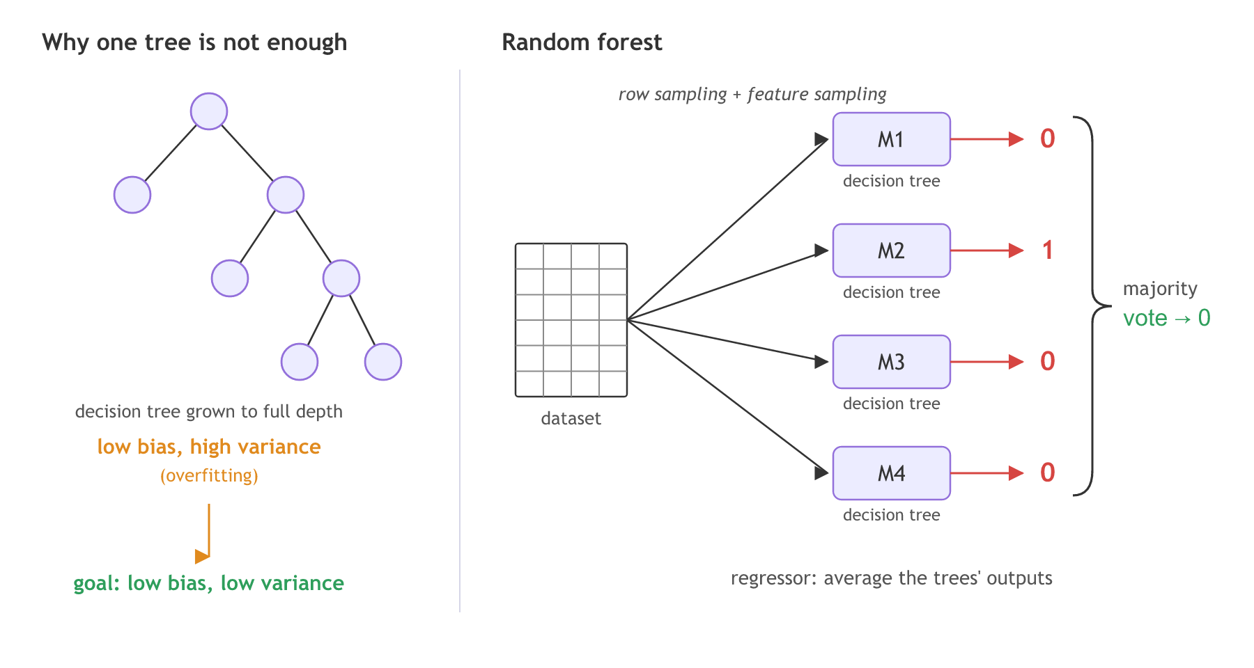
scikit-learn draws the feature sample at every split of a tree, not once per tree. The share is set by max_features; for the classifier the default is the square root of the number of features.
Comparing one deep tree with a forest
The breast cancer dataset has 569 tumours, 30 measurements each, labelled malignant or benign. One fully grown tree and a forest of 100 trees train on the same 70% and are tested on the same 30%.
Building the forest with RandomForestClassifier
from sklearn.ensemble import RandomForestClassifier

# 100 trees; each sees a bootstrap sample of rows, and each split tries sqrt(30) of the features
forest = RandomForestClassifier(n_estimators=100, max_features="sqrt", random_state=0)
forest.fit(X_train, y_train)
Measuring variance across ten splits
Variance is how much a model changes when the data changes. Training each model on ten different train and test splits and looking at the spread of its test accuracy measures it.
accs = []
for seed in range(10):
    a, b, c, d = train_test_split(X, y, test_size=0.3, random_state=seed)
    accs.append(Model(random_state=0).fit(a, c).score(b, d))
print(np.mean(accs), np.std(accs)) # the average and the spreadimport numpy as np
from sklearn.datasets import load_breast_cancer
from sklearn.model_selection import train_test_split
from sklearn.tree import DecisionTreeClassifier
from sklearn.ensemble import RandomForestClassifier
X, y = load_breast_cancer(return_X_y=True)
X_train, X_test, y_train, y_test = train_test_split(X, y, test_size=0.3, random_state=0)
tree = DecisionTreeClassifier(random_state=0).fit(X_train, y_train)
forest = RandomForestClassifier(n_estimators=100, max_features="sqrt", random_state=0)
forest.fit(X_train, y_train)
for name, m in [("one deep tree", tree), ("random forest", forest)]:
print(f"{name:14} train {m.score(X_train, y_train):.3f} test {m.score(X_test, y_test):.3f}")
for name, Model in [("one deep tree", DecisionTreeClassifier), ("random forest", RandomForestClassifier)]:
accs = []
for seed in range(10):
a, b, c, d = train_test_split(X, y, test_size=0.3, random_state=seed)
accs.append(Model(random_state=0).fit(a, c).score(b, d))
print(f"{name:14} 10 splits: mean {np.mean(accs):.3f}, spread {np.std(accs):.3f}")one deep tree train 1.000 test 0.912 random forest train 1.000 test 0.959 one deep tree 10 splits: mean 0.926, spread 0.017 random forest 10 splits: mean 0.960, spread 0.012
What the tree and the forest scores mean
- Both score 1.000 on the training data. Every tree in the forest is grown fully too, so low bias holds for both.
- The test accuracy differs: 0.912 for the tree, 0.959 for the forest. The gap between train and test is the overfitting the video describes.
- The spread over ten splits is 0.017 for the tree and 0.012 for the forest, and the forest's average is higher (0.960 against 0.926). That is the high variance turned into lower variance.
Answering the random forest interview questions
The video closes with the questions interviewers ask most often about random forests.
- Is normalisation needed for a random forest or a decision tree? No. A split compares one feature with a threshold, and scaling the feature moves the threshold with it, so the same rows land on each side.
- Is standardisation needed for KNN? Yes. K nearest neighbours (KNN) measures Euclidean or Manhattan distance, and a feature with large numbers takes over the distance.
- Is a random forest affected by outliers? Mostly no, for outliers in the features: a split only cares about the order of the values, so one huge value ends up on one side like any other large value. Outliers in the target of a
RandomForestRegressordo pull the average in their leaf. - Is KNN affected by outliers? Yes. An outlier sits among the neighbours of nearby points and shifts the distances.
Bagging is not limited to forests. A custom bagging model uses any combination of algorithms and combines their outputs, as the M1 to M4 example in Bagging and boosting did.
Scaling the features for a forest and for KNN
from sklearn.preprocessing import StandardScaler

scaler = StandardScaler().fit(X_train)         # learn the mean and std on the training rows
Xs_train, Xs_test = scaler.transform(X_train), scaler.transform(X_test)from sklearn.preprocessing import StandardScaler
from sklearn.neighbors import KNeighborsClassifier
scaler = StandardScaler().fit(X_train)
Xs_train, Xs_test = scaler.transform(X_train), scaler.transform(X_test)
for name, m in [("random forest", RandomForestClassifier(random_state=0)), ("KNN", KNeighborsClassifier())]:
raw = m.fit(X_train, y_train).score(X_test, y_test)
scaled = m.fit(Xs_train, y_train).score(Xs_test, y_test)
print(f"{name:13} raw {raw:.3f} scaled {scaled:.3f}")random forest raw 0.959 scaled 0.959 KNN raw 0.947 scaled 0.959
What scaling does to the forest and to KNN
- The forest scores 0.959 raw and scaled. Scaling changed every number in the data and none of the tree splits.
- KNN moves from 0.947 to 0.959 once the features are standardised, because its distances change.
RandomForestClassifier averages the trees' class probabilities instead and picks the class with the highest average (a soft vote). The answer is almost always the same; the difference shows only when the vote is close.Predicting used car prices with RandomForestRegressor
A random forest regressor is the same forest with one change: every tree predicts a number, and the forest returns the average of the trees' numbers. The used car dataset has 15,411 cars sold on cardekho.com, with each car's model, age, kilometres driven, seller type, fuel, transmission, mileage, engine, power, seats and its selling price in rupees. The task is to predict the selling price.
Loading the car data and encoding the text columns
The file loads from its URL. car_name and brand repeat what model already says, so they are dropped. model has 120 values and becomes one number per model (label encoding). Seller type, fuel type and transmission have 2 to 5 values each and become 0 or 1 columns (one-hot encoding). The forest needs no scaling.
url = ("https://raw.githubusercontent.com/krishnaik06/The-Grand-Complete-Data-Science-Materials/"
       "main/Machine%20Learning/8-Random%20Forest/Projects/data/cardekho_imputated.csv")
df = pd.read_csv(url, index_col=[0]).drop(columns=["car_name", "brand"])
df["model"] = df["model"].astype("category").cat.codes        # one number per car model
X = pd.get_dummies(df.drop(columns="selling_price"), drop_first=True,
                   columns=["seller_type", "fuel_type", "transmission_type"])
y = df["selling_price"]
Averaging the trees' prices for one car
A fitted forest keeps its trees in estimators_, so the average can be checked by hand.
forest = RandomForestRegressor(n_estimators=100, random_state=0).fit(X_train, y_train)
car = X_test.iloc[[0]].to_numpy()
each = [tree.predict(car)[0] for tree in forest.estimators_] # 100 prices for one carimport numpy as np
import pandas as pd
from sklearn.model_selection import train_test_split
from sklearn.linear_model import LinearRegression
from sklearn.tree import DecisionTreeRegressor
from sklearn.ensemble import RandomForestRegressor
url = ("https://raw.githubusercontent.com/krishnaik06/The-Grand-Complete-Data-Science-Materials/"
"main/Machine%20Learning/8-Random%20Forest/Projects/data/cardekho_imputated.csv")
df = pd.read_csv(url, index_col=[0]).drop(columns=["car_name", "brand"])
df["model"] = df["model"].astype("category").cat.codes # one number per car model
X = pd.get_dummies(df.drop(columns="selling_price"), drop_first=True,
columns=["seller_type", "fuel_type", "transmission_type"])
y = df["selling_price"]
X_train, X_test, y_train, y_test = train_test_split(X, y, test_size=0.2, random_state=42)
print("cars:", len(df), " columns after encoding:", X.shape[1])
models = {"linear regression": LinearRegression(),
"one deep tree": DecisionTreeRegressor(random_state=0),
"random forest": RandomForestRegressor(n_estimators=100, random_state=0)}
for name, m in models.items():
m.fit(X_train, y_train)
print(f"{name:17} train R2 {m.score(X_train, y_train):.3f} test R2 {m.score(X_test, y_test):.3f}")
forest = models["random forest"]
car = X_test.iloc[[0]].to_numpy()
each = [tree.predict(car)[0] for tree in forest.estimators_]
print("first four trees for the first test car:", [int(v) for v in each[:4]])
print("mean of the 100 trees:", int(np.mean(each)), " forest prediction:", int(forest.predict(car)[0]))
print("true price:", int(y_test.iloc[0]))cars: 15411 columns after encoding: 14 linear regression train R2 0.622 test R2 0.665 one deep tree train R2 0.999 test R2 0.880 random forest train R2 0.981 test R2 0.931 first four trees for the first test car: [211000, 211000, 235000, 335000] mean of the 100 trees: 246180 forest prediction: 246180 true price: 190000
What the car price models show
- Linear regression scores a test R² of 0.665: one straight line cannot follow how the price depends on the model, age and power together.
- One deep tree fits the training cars almost exactly (0.999) and drops to 0.880 on the test cars, the low bias and high variance of a single tree.
- The forest scores 0.931 on the test cars, the best of the three, with a training R² of 0.981.
- The trees disagree about the first test car (211,000, 211,000, 235,000 and 335,000 rupees from the first four), and the mean of all 100 trees, 246,180, is exactly the forest's prediction. The car sold for 190,000.
Scoring a forest with out-of-bag rows
Each tree's bootstrap sample makes as many draws as there are rows, d, but with replacement: some rows are drawn twice and others never. The rows a tree never draws are its out-of-bag (OOB) rows. They work like a validation set for that tree. Scoring every training row with only the trees that did not train on it gives the out-of-bag score, a test score that needs no rows set aside.
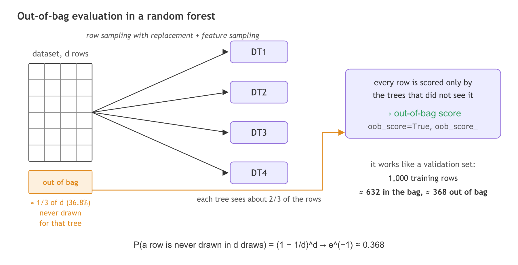
How many rows stay out? One draw misses a given row with probability 1 − 1/d, so all d draws miss it with probability (1 − 1/d)d. For a large d this tends to e−1 ≈ 0.368: about 63.2% of the rows go into the bag and 36.8% stay out. The board rounds it to one third, as in a split of 1,000 training rows into 2/3 for training and 1/3 for validation.
Counting the rows a bootstrap sample leaves out
import numpy as np

rng = np.random.default_rng(0)
for d in (10, 100, 1000, 10000):
    rows = rng.choice(d, size=d, replace=True)          # one bootstrap sample of d draws
    oob = d - len(np.unique(rows))                      # rows that were never drawn
    print(f"d = {d:>5}: out of bag {oob:>4} rows = {oob / d:.3f}   formula {(1 - 1 / d) ** d:.3f}")
print("e^-1 =", round(float(np.exp(-1)), 3))d = 10: out of bag 3 rows = 0.300 formula 0.349 d = 100: out of bag 37 rows = 0.370 formula 0.366 d = 1000: out of bag 370 rows = 0.370 formula 0.368 d = 10000: out of bag 3658 rows = 0.366 formula 0.368 e^-1 = 0.368
Reading oob_score_ on the car forest
oob_score=True makes the forest remember which rows each tree left out. After fitting, oob_score_ holds the R² of the out-of-bag predictions and oob_prediction_ the predictions themselves, all computed from the training rows alone.
from sklearn.ensemble import RandomForestRegressor
from sklearn.metrics import mean_absolute_error

forest = RandomForestRegressor(n_estimators=100, oob_score=True, random_state=0)
forest.fit(X_train, y_train)
oob_mae = mean_absolute_error(y_train, forest.oob_prediction_)
test_mae = mean_absolute_error(y_test, forest.predict(X_test))
print(f"out-of-bag: R2 {forest.oob_score_:.3f}   MAE {oob_mae:,.0f}")
print(f"test:       R2 {forest.score(X_test, y_test):.3f}   MAE {test_mae:,.0f}")
print(f"most expensive car: training rows {y_train.max():,} test rows {y_test.max():,}")out-of-bag: R2 0.843 MAE 102,415 test: R2 0.931 MAE 101,812 most expensive car: training rows 39,500,000 test rows 13,000,000
What the out-of-bag numbers show
- The share left out settles at 0.368: 370 of 1,000 rows and 3,658 of 10,000, the e−1 of the formula. With only 10 rows the share is rough (3 rows here, against 0.349 from the formula).
- The out-of-bag MAE, 102,415 rupees, is close to the test MAE of 101,812, so the training rows alone gave a fair estimate of the typical error on new cars.
- The out-of-bag R² is lower, 0.843 against 0.931. The training rows hold the most expensive car, 39,500,000 rupees, and the test rows stop at 13,000,000. R² squares the errors, so a few very expensive training cars weigh heavily in it, while the typical error in rupees is about the same.
Random forest vs one decision tree
| One decision tree | Random forest | |
|---|---|---|
| Bias and variance | low bias, high variance | low bias, lower variance |
| Data per tree | all rows, all features | bootstrap rows, a sample of features at each split |
| Breast cancer test accuracy | 0.912 | 0.959 |
| Used car price test R² | 0.880 | 0.931 |
| Can you read it? | yes, a white box model | no, 100 trees make a black box model |
| Training time | one tree | about n_estimators times one tree |
Where you use a random forest
- A first strong model on tabular data, since it needs no scaling and little tuning.
- Feature importance:
forest.feature_importances_ranks which columns the splits used most. - Data with outliers in the features, where distance-based models such as KNN struggle.
oob_score_, and tune max_depth or min_samples_leaf if the gap is large.Related
- Previous: Bagging and boosting
- Next: AdaBoost
- See also: Decision tree in scikit-learn
- Reference: RandomForestClassifier in the scikit-learn API
- Change
max_features="sqrt"tomax_features=Noneso every split sees all 30 features, and compare the forest's test accuracy. - Set
n_estimators=300in the out-of-bag forest and check whetheroob_score_moves away from 0.843. - Print
forest.feature_importances_.argmax()to find the feature the trees used most.
You understood something today that you didn't yesterday.