Decision tree in scikit-learn
DecisionTreeClassifier is the scikit-learn class that builds a classification tree, and plot_tree draws the fitted tree with each node's question, Gini impurity, sample count and class counts.
Last updated: 04 Oct, 2026 · scikit-learn 1.9.1
Decision tree regression and pruning ended the hand-worked part of trees. The video's notebook fits a tree on the Iris flowers and draws it, so the questions, Gini values and class counts from the earlier tree lessons all show up on one picture.
Reading the DecisionTreeClassifier parameters
The video plans to let the tree overfit first and prune it afterwards, so it keeps the defaults and walks through the parameters:
- criterion: the impurity measure,
"gini"by default;"entropy"and"log_loss"use entropy. - splitter:
"best"tries every candidate split;"random"picks among random ones. The video recommends best. - max_depth, min_samples_leaf and max_features: hyperparameters that limit how far the tree grows and how many features each split looks at.
The dataset is Iris: 150 flowers, 50 of each species (setosa, versicolor, virginica), with four measurements each: sepal length, sepal width, petal length and petal width.
Fitting and drawing the Iris tree
Loading Iris
import matplotlib.pyplot as plt
from sklearn import tree
from sklearn.datasets import load_iris
from sklearn.tree import DecisionTreeClassifier

iris = load_iris()           # 150 flowers, 4 measurements, 3 species
Fitting the classifier
# Default settings: criterion="gini", splitter="best", no depth limit
classifier = DecisionTreeClassifier(random_state=0)
classifier.fit(iris.data, iris.target)
The video's first attempt calls tree.plot, which does not exist, then plots before fitting and gets a NotFittedError. The working order is fit first, then tree.plot_tree. The video's call passes only filled=True, so its nodes read X[0] to X[3]; feature_names and class_names are added here, and random_state=0 makes the tie-breaks repeat.
plt.figure(figsize=(15, 10))
tree.plot_tree(classifier, filled=True, feature_names=iris.feature_names,
               class_names=list(iris.target_names))
plt.title("Decision tree on the Iris dataset")
plt.show()
print("depth:", classifier.get_depth(), " leaves:", classifier.get_n_leaves())
print("root gini:", round(classifier.tree_.impurity[0], 3))depth: 5 leaves: 9 root gini: 0.667
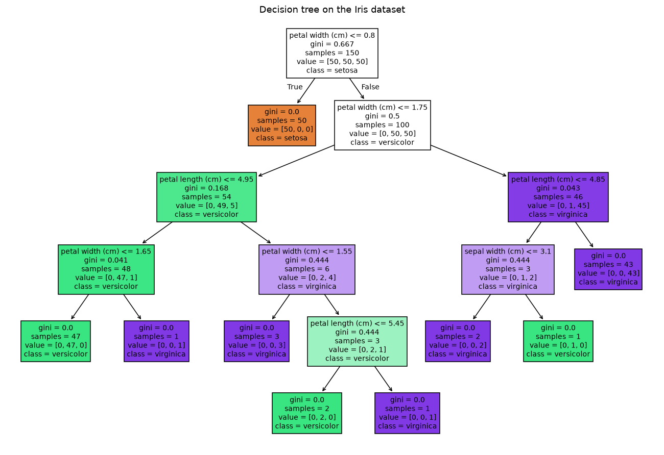
Reading the Iris tree
- The root asks petal width ≤ 0.8 on all 150 samples, value [50, 50, 50], gini 0.667.
- The left branch is a leaf: 50 samples, value [50, 0, 0], gini 0.0. One question separates all the setosa flowers.
- The right branch holds the other 100 flowers, [0, 50, 50], gini 0.5, and splits on petal width ≤ 1.75 into [0, 49, 5] and [0, 1, 45].
- Deep in the tree a node holds [0, 47, 1]. The video asks whether such a split is worth making at all: one flower out of 48 is a lot of tree for little gain. That is the post-pruning question.
The clip names the left leaf versicolor; value [50, 0, 0] is class 0, setosa. The root's gini of 0.667 is above the 0.5 ceiling from Entropy and Gini impurity because Iris has three classes: 1 − 3 × (1/3)² = 0.667. The 0.5 ceiling holds for two classes, which is why the node with only versicolor and virginica shows exactly 0.5.
Testing the tree with a confusion matrix
The video fits the tree on all 150 flowers and never tests it. Holding out 30 flowers (20%) as a test set shows how the full tree does on flowers it never saw. A Confusion matrix and the classification report then show which species it mixes up.
Holding out a test set
from sklearn.model_selection import train_test_split
from sklearn.metrics import confusion_matrix, classification_report, accuracy_score

# 120 flowers to train on, 30 to test on
X_train, X_test, y_train, y_test = train_test_split(iris.data, iris.target, test_size=0.2, random_state=10)
tree_classifier = DecisionTreeClassifier(random_state=0).fit(X_train, y_train)y_pred = tree_classifier.predict(X_test)
print("depth:", tree_classifier.get_depth(), " leaves:", tree_classifier.get_n_leaves(),
" train accuracy:", tree_classifier.score(X_train, y_train))
print(confusion_matrix(y_test, y_pred))
print(classification_report(y_test, y_pred, target_names=iris.target_names))depth: 6 leaves: 10 train accuracy: 1.0
[[10 0 0]
[ 0 12 1]
[ 0 0 7]]
precision recall f1-score support
setosa 1.00 1.00 1.00 10
versicolor 1.00 0.92 0.96 13
virginica 0.88 1.00 0.93 7
accuracy 0.97 30
macro avg 0.96 0.97 0.96 30
weighted avg 0.97 0.97 0.97 30Pre-pruning the Iris tree with GridSearchCV
Pre-pruning limits the tree while it grows, as in Decision tree regression and pruning. GridSearchCV tries every mix of criterion, splitter, depth and max_features with 5-fold cross-validation on the 120 training flowers, and keeps the best. Older code for this grid lists max_features="auto", which scikit-learn removed in 1.3; None (all features) stands in for it.
from sklearn.model_selection import GridSearchCV

param = {
    "criterion": ["gini", "entropy", "log_loss"],
    "splitter": ["best", "random"],
    "max_depth": [1, 2, 3, 4, 5],
    "max_features": [None, "sqrt", "log2"],
}
grid = GridSearchCV(DecisionTreeClassifier(random_state=0), param_grid=param, cv=5, scoring="accuracy")
grid.fit(X_train, y_train)print("best params:", grid.best_params_)
print("best cv accuracy:", round(grid.best_score_, 3))
best = grid.best_estimator_
print("depth:", best.get_depth(), " leaves:", best.get_n_leaves())
y_pred = grid.predict(X_test)
print(confusion_matrix(y_test, y_pred))
print("test accuracy:", round(accuracy_score(y_test, y_pred), 3))best params: {'criterion': 'gini', 'max_depth': 3, 'max_features': None, 'splitter': 'random'}
best cv accuracy: 0.967
depth: 3 leaves: 5
[[10 0 0]
[ 0 13 0]
[ 0 0 7]]
test accuracy: 1.0What the test and the grid search show
- The full tree has depth 6 and 10 leaves and a training accuracy of 1.0: every training flower is classified right, a sign of overfitting.
- On the 30 test flowers it makes one mistake: the confusion matrix shows one versicolor predicted as virginica, so versicolor recall is 12/13 = 0.92 and virginica precision 7/8 = 0.88, for an accuracy of 0.97.
- The grid search picks gini, max_depth 3, the random splitter and all features, with a cross-validation accuracy of 0.967 on the training flowers. The tree it keeps has 5 leaves, half as many.
- The grid-searched tree gets all 30 test flowers right. On 30 flowers one mistake is 0.033 of accuracy, so the cross-validation score, which averages five folds, is the steadier guide; the test set checks the choice once.
Full tree vs grid-searched tree
| Full tree (defaults) | Grid-searched tree | |
|---|---|---|
| Depth and leaves | 6 and 10 | 3 and 5 |
| Chosen by | The defaults: grow until every leaf is pure | 5-fold cross-validation over 90 settings |
| Training accuracy | 1.0 | Below 1.0 is allowed |
| Test accuracy (30 flowers) | 0.97, one versicolor called virginica | 1.0 |
| Readable with plot_tree | Yes, but crowded | Yes, at a glance |
| Risk | Overfitting | Underfitting if the depth is too small |
Where you use plot_tree
- Explaining a model: the drawing shows every question the model asks and how many training rows reach each node.
- Spotting overfitting: leaves with 1 or 2 samples, such as [0, 0, 1], are splits made for single rows.
- Checking a pruning choice: draw the tree before and after setting
max_depthorccp_alpha.
random_state, two runs can choose different splits when features tie, so the drawing and the scores can change between runs. A deep tree also turns into an unreadable plot: pass max_depth=2 to plot_tree to draw only the top, or print the rules with export_text.Related
- Previous: Decision tree regression and pruning
- Next: Bagging and boosting
- Reference: plot_tree in the scikit-learn API reference
- Fit the Iris tree with
criterion="entropy"and plot it. What does the root's impurity read now (log₂ 3 for three equal classes)? - Draw only the top of the tree with
tree.plot_tree(classifier, max_depth=2, filled=True). - Print the rules as text with
print(export_text(classifier, feature_names=iris.feature_names))(importexport_textfromsklearn.tree).
Every expert started right here.