Gradient boosting
Gradient boosting is a boosting algorithm that starts from the average of the target and adds decision trees one after another, each trained on the residuals of the model so far and scaled down by a learning rate.
Last updated: 05 Oct, 2026 · scikit-learn 1.9.1
AdaBoost made the next stump focus on the records the last one got wrong by raising their weights. Gradient boosting hands the next tree the errors themselves. The XGBoost classifier and XGBoost regressor are an optimised form of it, so the steps here are the ones those lessons build on.
Starting from the average salary
The worked example predicts salary from experience and degree. Gradient boosting works for regression and for classification; the regression form is the easiest to follow by hand.
| Exp | Degree | Salary | Base model ŷ | Residual R1 |
|---|---|---|---|---|
| 2 | B.E | 50K | 75K | −25K |
| 3 | Masters | 70K | 75K | −5K |
| 5 | Masters | 80K | 75K | 5K |
| 6 | PhD | 100K | 75K | 25K |
Step 1 creates a base model that predicts the average for every record: (50 + 70 + 80 + 100) / 4 = 75K. Step 2 computes the residuals, the error of that prediction: R1 = y − ŷ, so −25, −5, 5 and 25.
Fitting a tree to the residuals
Step 3 trains a decision tree DT1 with experience and degree as the inputs and R1 as the target. Say the tree predicts the residuals as −23, −3, 3 and 20: close to −25, −5, 5 and 25, but not equal, as a small tree's leaves rarely are.
Adding the tree's output in full gives 75 + (−23) = 52 for the first record, almost its 50K. The video calls this overfitting: a fit this close to the training data has low bias but high variance, so new data gets worse predictions. So each tree's output is multiplied by a learning rate α between 0 and 1. With α = 0.1 the first record becomes 75 + 0.1 × (−23) = 72.7 and the second 75 + 0.1 × (−3) = 74.7. The new residuals, R2, are the targets of the next tree DT2. The video works the first record out as 73.7; 75 − 2.3 is 72.7.
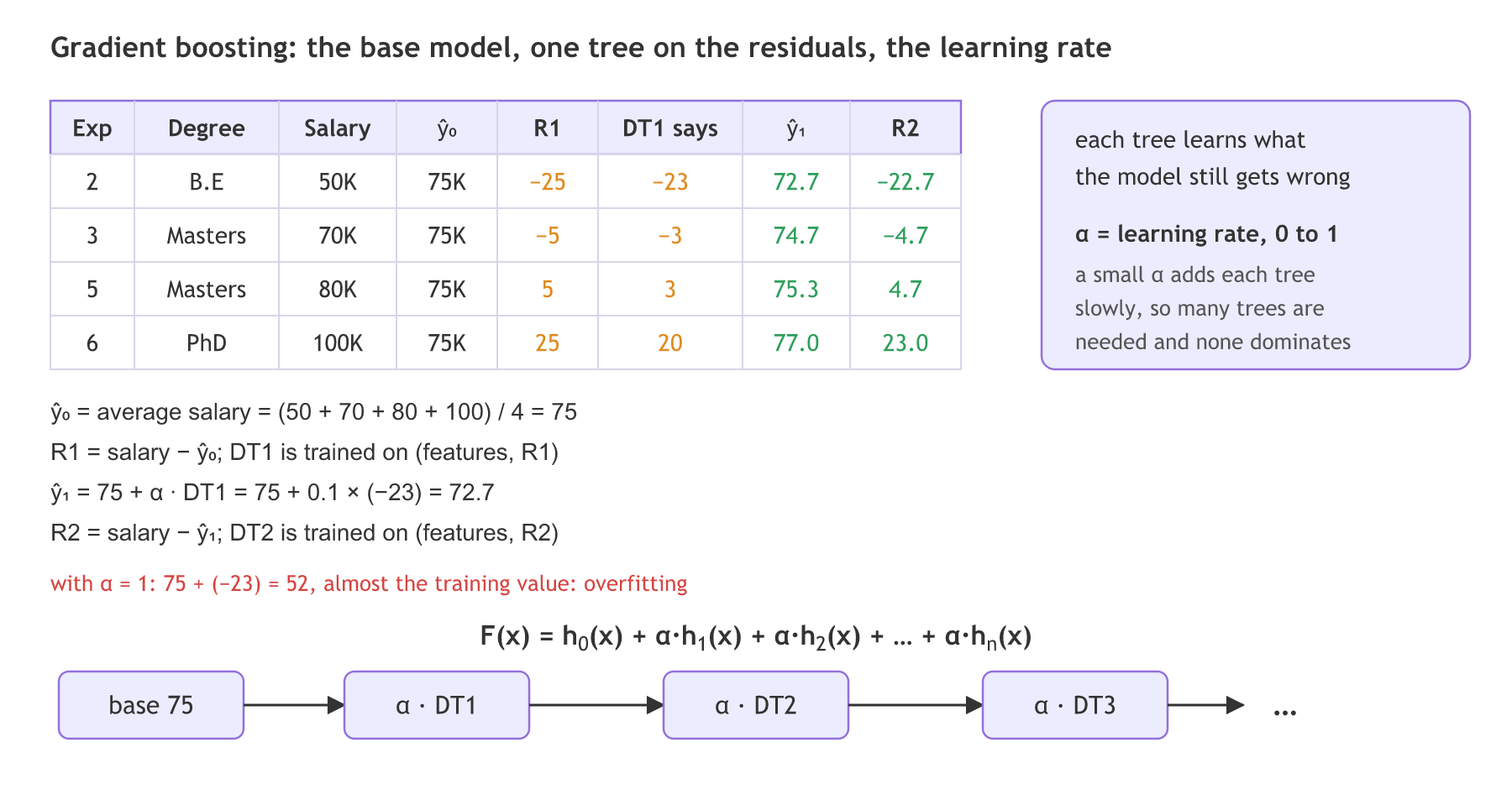
| Salary | ŷ after DT1 | R2 = salary − ŷ |
|---|---|---|
| 50K | 75 + 0.1 × (−23) = 72.7 | −22.7 |
| 70K | 75 + 0.1 × (−3) = 74.7 | −4.7 |
| 80K | 75 + 0.1 × 3 = 75.3 | 4.7 |
| 100K | 75 + 0.1 × 20 = 77.0 | 23.0 |
Every residual moved a little toward 0. Each new tree trains on the latest residuals and adds a small step, so the model reaches the targets slowly, over many trees.
Writing the final function
The model is the base model h₀ plus every tree hᵢ, each scaled by the learning rate:
The video writes h₀(x) + α₁h₁(x) + … + αₙhₙ(x), one α per tree. In scikit-learn the base model is added once, unscaled, and one learning_rate is shared by every tree.
Seeing the residual as a gradient
The name comes from the loss. For the squared error L = ½(y − F)², the derivative with respect to the prediction F is −(y − F). The video works it on three records with salaries 50, 70 and 60K: the base model predicts their mean, 60, so the residuals are −10, 10 and 0. The residual is the negative gradient, so each tree takes one step downhill, like Gradient descent, but on the predictions instead of on a weight. The video calls it the pseudo-residual, and a different loss gives a different one: for log loss in classification it is label − probability, the residual of the XGBoost classifier.
Running three rounds by hand and with GradientBoostingRegressor
A depth-1 tree fitted to the residuals, three times, with α = 0.1, on the four records. The trees here are real fits, so their outputs are not the board's assumed −23, −3, 3 and 20.
One round of gradient boosting
F = np.full(len(salary), salary.mean())          # base model: the average, 75
r = salary - F                                   # residuals
tree = DecisionTreeRegressor(max_depth=1).fit(X, r)
F = F + 0.1 * tree.predict(X)                    # add the tree's output times the learning rate
GradientBoostingRegressor with the same settings
staged_predict yields the predictions after one tree, two trees, three trees, and so on.
from sklearn.ensemble import GradientBoostingRegressor

gbr = GradientBoostingRegressor(n_estimators=3, learning_rate=0.1, max_depth=1).fit(X, salary)
stages = list(gbr.staged_predict(X)) # predictions after 1, 2 and 3 treesimport numpy as np
from sklearn.tree import DecisionTreeRegressor
from sklearn.ensemble import GradientBoostingRegressor
X = np.array([[2, 0], [3, 1], [5, 1], [6, 2]]) # experience, degree (0 = B.E, 1 = Masters, 2 = PhD)
salary = np.array([50.0, 70, 80, 100])
F = np.full(len(salary), salary.mean())
print("base model:", F)
for round_ in (1, 2, 3):
r = salary - F
tree = DecisionTreeRegressor(max_depth=1).fit(X, r)
F = F + 0.1 * tree.predict(X)
print(f"round {round_}: residuals {r.round(2)} tree says {tree.predict(X).round(2)} new prediction {F.round(2)}")
gbr = GradientBoostingRegressor(n_estimators=3, learning_rate=0.1, max_depth=1).fit(X, salary)
stages = list(gbr.staged_predict(X))
print("GradientBoostingRegressor after 3 trees:", stages[-1].round(2))
print("same as by hand:", np.allclose(stages[-1], F))base model: [75. 75. 75. 75.] round 1: residuals [-25. -5. 5. 25.] tree says [-15. -15. 15. 15.] new prediction [73.5 73.5 76.5 76.5] round 2: residuals [-23.5 -3.5 3.5 23.5] tree says [-23.5 7.83 7.83 7.83] new prediction [71.15 74.28 77.28 77.28] round 3: residuals [-21.15 -4.28 2.72 22.72] tree says [-7.57 -7.57 -7.57 22.72] new prediction [70.39 73.53 76.53 79.55] GradientBoostingRegressor after 3 trees: [70.39 73.53 76.53 79.55] same as by hand: True
What the three rounds show
- The base model predicts 75 for every record, and the first residuals are the board's −25, −5, 5 and 25.
- The first tree splits experience between 3 and 5 and predicts −15 and 15, the average residual on each side. With α = 0.1 the predictions move from 75 to 73.5 and 76.5.
- Each round shrinks the residuals a little: −25 becomes −23.5 and then −21.15, and 25 becomes 23.5 and then 22.72. Three trees with α = 0.1 are still far from the salaries, which is why gradient boosting uses many trees.
- GradientBoostingRegressor gives the same predictions after three trees, 70.39, 73.53, 76.53 and 79.55, so the hand loop is the algorithm.
Predicting used car prices with gradient boosting
The used car data from Random forest, loaded and split the same way. The forest scored a test R² of 0.931 there. Gradient boosting with depth-3 trees and α = 0.1 runs for 300 trees, and staged_predict scores it after 1, 10, 100 and 300 of them.
from sklearn.ensemble import GradientBoostingRegressor
from sklearn.metrics import r2_score

gbr = GradientBoostingRegressor(n_estimators=300, learning_rate=0.1, max_depth=3, random_state=0)
gbr.fit(X_train, y_train)
stages = list(gbr.staged_predict(X_test))
for n in (1, 10, 100, 300):
    print(f"{n:3} trees: test R2 {r2_score(y_test, stages[n - 1]):.3f}")
print(f"train R2 after 300 trees: {gbr.score(X_train, y_train):.3f}")1 trees: test R2 0.118 10 trees: test R2 0.668 100 trees: test R2 0.912 300 trees: test R2 0.933 train R2 after 300 trees: 0.971
Reading the car price scores
- One tree scores 0.118: with α = 0.1 it moves every price only a tenth of the way from the average.
- 10 trees reach 0.668 and 100 trees 0.912; each tree fixes part of what the earlier ones left.
- 300 trees score 0.933, level with the random forest's 0.931, with a training R² of 0.971. The gap between train and test is small, so these 300 trees have not started to overfit.
Gradient boosting vs AdaBoost
| Gradient boosting | AdaBoost | |
|---|---|---|
| What the next tree learns | the residuals of the model so far | the same records, reweighted toward mistakes |
| Base model | the average of the target (regression) | none; the first stump starts the chain |
| Trees | small trees, often depth 3 | stumps of depth 1 |
| Combining | base + learning rate × each tree's output | vote weighted by each stump's performance |
| scikit-learn | GradientBoostingRegressor, GradientBoostingClassifier | AdaBoostRegressor, AdaBoostClassifier |
Where you use gradient boosting
- Price and demand prediction on tabular data, such as the used car prices above.
- Ranking and click prediction, where many weak signals across columns add up.
- A step before XGBoost or LightGBM: the same idea with fewer settings, in scikit-learn itself.
n_iter_no_change so training stops when a validation score stops improving.Related
- Previous: AdaBoost
- Next: XGBoost classifier
- See also: Gradient descent
- Reference: scikit-learn user guide, Gradient-boosted trees
- Change
0.1to1.0in the hand loop and see how close round 1 gets to the salaries. - Set
max_depth=2in the hand loop and in GradientBoostingRegressor, and check they still match. - Set
learning_rate=0.5on the car data and compare the test R² after 10 trees.
This is what real progress feels like.