XGBoost regressor
The XGBoost regressor is the regression form of XGBoost: it starts from the average of the target, then adds binary trees one after another, each fitted to the residuals and split by the gain in similarity weight.
Last updated: 05 Oct, 2026 · XGBoost 3.4.1
The XGBoost classifier started from a probability of 0.5. The regressor starts, like Gradient boosting, from the average of the target, and follows the same steps as the classifier with numbers: residuals, similarity weights and gain, with a simpler similarity formula.
Starting from the average salary
The video predicts salary (in thousands) from years of experience and whether the person had a gap in their career.
| Experience | Gap | Salary | Residual |
|---|---|---|---|
| 2 | Yes | 40K | −11 |
| 2.5 | Yes | 42K | −9 |
| 3 | No | 52K | 1 |
| 4 | No | 60K | 9 |
| 4.5 | Yes | 62K | 11 |
The base model outputs the average salary for every input: 51K. Each residual is the salary minus 51. The root of the first tree holds all five: [−11, −9, 1, 9, 11].
The video first writes 41K in the second row, which makes the average exactly 51, and then changes it to 42K to make the arithmetic easier while keeping 51 as the base. With 42K the average is 51.2, so the residuals add up to 1 instead of 0. The numbers here follow the board: 42K with a base of 51.
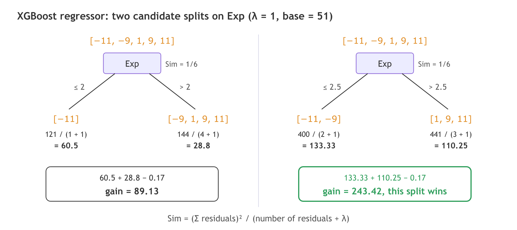
The first split is on experience, a continuous feature, so it is a threshold: ≤2 and >2. The left branch gets [−11], the right branch [−9, 1, 9, 11].
Calculating the similarity weight with λ = 1
For regression the bottom of the similarity weight is the number of residuals plus λ. A larger λ penalises the similarity more. The video first works the left leaf with λ = 0, which gives 121 / 1 = 121, then sets λ = 1 for the rest.
- ≤2: (−11)² / (1 + 1) = 121 / 2 = 60.5.
- >2: (−9 + 1 + 9 + 11)² / (4 + 1) = 144 / 5 = 28.8.
- Root: (−11 − 9 + 1 + 9 + 11)² / (5 + 1) = 1 / 6 ≈ 0.17.
The board writes 121 / 2 as 65.5 and the gain as 98.34. It corrects 65.5 to 60.5 but not the gain; with 60.5 the gain is 89.13, the number the video says aloud.
Choosing the better split at 2.5
The next candidate threshold is ≤2.5 and >2.5. The left branch gets [−11, −9]: (−20)² / (2 + 1) = 400 / 3 = 133.33. The right branch gets [1, 9, 11]: 21² / (3 + 1) = 441 / 4 = 110.25. The gain is 133.33 + 110.25 − 0.17 = 243.42, far above 89.13, so the tree splits at 2.5.
Predicting a salary from the base value and the trees
A new record starts at the base value 51, then follows the tree and adds the learning rate times the leaf's value. More trees add more terms: 51 + α₁·tree₁ + α₂·tree₂ + … + αₙ·treeₙ.
The video uses the average of each leaf as its value: −10 for [−11, −9] and 7 for [1, 9, 11]. XGBoost's leaf output divides by the count plus λ, so with λ = 1 the values are −20 / 3 = −6.67 and 21 / 4 = 5.25. The video's averages are the leaf outputs for λ = 0. The library also uses one learning rate for all trees.
Computing every split of the salary table
The table typed in and a loop over the four thresholds between the experience values.
The similarity weight for regression
base = 51                       # the board's base model output
res = salary - base
lam = 1

def sim(r):
return r.sum() ** 2 / (len(r) + lam) # (sum of residuals)^2 / (count + lambda)import numpy as np
exp = np.array([2, 2.5, 3, 4, 4.5])
salary = np.array([40, 42, 52, 60, 62])
base = 51
res = salary - base
lam = 1
def sim(r):
return r.sum() ** 2 / (len(r) + lam)
print("residuals:", res, " root similarity:", round(sim(res), 3))
for t in (2, 2.5, 3, 4):
left, right = res[exp <= t], res[exp > t]
print(f"Exp <= {t:<3} left {sim(left):6.2f} right {sim(right):6.2f} gain {sim(left) + sim(right) - sim(res):6.2f}")
left, right = res[exp <= 2.5], res[exp > 2.5]
print("leaf outputs (lambda = 1):", round(left.sum() / (len(left) + lam), 2), round(right.sum() / (len(right) + lam), 2))
print("leaf averages (the video):", left.mean(), right.mean())residuals: [-11 -9 1 9 11] root similarity: 0.167 Exp <= 2 left 60.50 right 28.80 gain 89.13 Exp <= 2.5 left 133.33 right 110.25 gain 243.42 Exp <= 3 left 90.25 right 133.33 gain 223.42 Exp <= 4 left 20.00 right 60.50 gain 80.33 leaf outputs (lambda = 1): -6.67 5.25 leaf averages (the video): -10.0 7.0
What the four candidate splits show
- The ≤2 split gives 60.5, 28.8 and a gain of 89.13; the ≤2.5 split gives 133.33, 110.25 and 243.42, the board's corrected numbers.
- The ≤3 split scores 223.42 and ≤4 only 80.33, so 2.5 is the best threshold of the four.
- The leaf outputs are −6.67 and 5.25 with λ = 1, smaller than the averages −10 and 7.
Splitting on gap and computing the second-round residuals
The right branch [1, 9, 11] can be split again, on gap: Yes gets [11] (record 5) and No gets [1, 9] (records 3 and 4). With the board's leaf values, the average residual in each leaf, the first tree outputs −10, 11 and 5. With a learning rate of 0.1 the predictions are 51 + 0.1 × (−10) = 50.0 for records 1 and 2, 51 + 0.1 × 5 = 51.5 for records 3 and 4, and 51 + 0.1 × 11 = 52.1 for record 5.
![The first XGBoost regressor tree splits experience at 2.5 and the right branch on gap: the leaves hold the residuals [−11, −9], [11] and [1, 9] with values −10, 11 and 5; with a learning rate of 0.1 the predictions are 50.0, 50.0, 51.5, 51.5 and 52.1, leaving second-round residuals of −10, −8, 0.5, 8.5 and 9.9.](https://d14omfvx1qlabb.cloudfront.net/krishnaik.in/media/tutorials/machine-learning/b6ae7f7b69c041a582ca0538ee1eaf50.png)
The new residuals, salary minus prediction, are −10, −8, 0.5, 8.5 and 9.9. Each one is a little closer to 0 than the first round's −11, −9, 1, 9 and 11, and the second tree is trained on them.
λ also decides whether a split is made at all. With λ = 1 the gap split scores 121/2 + 100/3 − 441/4 = 60.5 + 33.33 − 110.25 = −16.42. A negative gain means the split makes the tree worse, so XGBoost keeps [1, 9, 11] as one leaf or splits it another way. With λ = 0 the same split gains 121 + 50 − 147 = 24.
The second round and the gap split as code
gap = np.array([1, 1, 0, 0, 1])                                       # 1 = Yes
leaf = np.where(exp <= 2.5, -10.0, np.where(gap == 1, 11.0, 5.0))      # the board's leaf values
pred = base + 0.1 * leaf                                              # learning rate 0.1
res2 = salary - pred # the targets of tree 2gap = np.array([1, 1, 0, 0, 1])
leaf = np.where(exp <= 2.5, -10.0, np.where(gap == 1, 11.0, 5.0))
pred = base + 0.1 * leaf
res2 = salary - pred
print("predictions after tree 1:", pred)
print("second-round residuals: ", res2)
right, g = res[exp > 2.5], gap[exp > 2.5]
for lam_value in (1, 0):
s = lambda r: r.sum() ** 2 / (len(r) + lam_value)
print(f"lambda = {lam_value}: gain of the gap split {s(right[g == 1]) + s(right[g == 0]) - s(right):.2f}")predictions after tree 1: [50. 50. 51.5 51.5 52.1] second-round residuals: [-10. -8. 0.5 8.5 9.9] lambda = 1: gain of the gap split -16.42 lambda = 0: gain of the gap split 24.00
What the second round shows
- The predictions are 50, 50, 51.5, 51.5 and 52.1, and the residuals −10, −8, 0.5, 8.5 and 9.9, the numbers in the diagram.
- With λ = 1 the gap split has a gain of −16.42, so XGBoost would not make it; with λ = 0 it gains 24. The board's tree uses the averages, which are the λ = 0 leaf values.
Fitting XGBRegressor on the salary table
XGBRegressor comes from the same xgboost package as the classifier; Installing scikit-learn has the install line and the extra brew install libomp step on macOS.
Matching the board with one tree of depth 1
base_score=51 is the base model, reg_lambda=1 is λ, and learning_rate=1.0 keeps the leaf values unscaled so they match the formula. max_depth=1 allows one split. Left unset, base_score would be estimated from the data as the mean, 51.2.
from xgboost import XGBRegressor

reg = XGBRegressor(n_estimators=1, max_depth=1, learning_rate=1.0, reg_lambda=1,
                   base_score=51, tree_method="exact")
reg.fit(X, salary)import pandas as pd
from xgboost import XGBRegressor
X = pd.DataFrame({"exp": exp, "gap": [1, 1, 0, 0, 1]}) # gap: 1 = Yes, 0 = No
reg = XGBRegressor(n_estimators=1, max_depth=1, learning_rate=1.0, reg_lambda=1,
base_score=51, tree_method="exact")
reg.fit(X, salary)
print(reg.get_booster().get_dump(with_stats=True)[0])
print("predictions:", reg.predict(X).round(2))
for lam_value in (0, 1, 10):
r = XGBRegressor(n_estimators=1, max_depth=1, learning_rate=1.0, reg_lambda=lam_value,
base_score=51, tree_method="exact").fit(X, salary)
print(f"reg_lambda={lam_value:<3} leaf outputs {np.round(r.predict(X)[[0, 4]] - 51, 2)}")0:[exp<2.75] yes=1,no=2,missing=1,gain=243.416656,cover=5 1:leaf=-6.66666651,cover=2 2:leaf=5.25,cover=3 predictions: [44.33 44.33 56.25 56.25 56.25] reg_lambda=0 leaf outputs [-10. 7.] reg_lambda=1 leaf outputs [-6.67 5.25] reg_lambda=10 leaf outputs [-1.67 1.62]
What the one-tree regressor printed
- The split is exp < 2.75 with gain 243.4. XGBoost places the threshold halfway between 2.5 and 3, the same partition as ≤2.5, and its gain is the board's 243.42.
- The leaves are −6.67 and 5.25, so the predictions are 51 − 6.67 = 44.33 and 51 + 5.25 = 56.25.
- λ shrinks the leaves: with λ = 0 they are −10 and 7, the video's averages; with λ = 10 they fall to −1.67 and 1.62.
Predicting diabetes progression with more and more trees
On the diabetes dataset (442 patients, 10 measurements, a disease progression score) the number of trees decides how far the boosting goes. r2_score takes the true values first.
from sklearn.datasets import load_diabetes
from sklearn.model_selection import train_test_split
from sklearn.metrics import r2_score
from xgboost import XGBRegressor

X, y = load_diabetes(return_X_y=True)
X_train, X_test, y_train, y_test = train_test_split(X, y, test_size=0.3, random_state=0)
for n in (1, 10, 100, 300):
    reg = XGBRegressor(n_estimators=n, max_depth=2, learning_rate=0.1, reg_lambda=1,
                       random_state=0).fit(X_train, y_train)
print(f"{n:3} trees: test R2 {r2_score(y_test, reg.predict(X_test)):.3f}")1 trees: test R2 0.079 10 trees: test R2 0.337 100 trees: test R2 0.340 300 trees: test R2 0.260
Reading the R2 scores
- One tree scores 0.079: with a learning rate of 0.1 it moves the predictions only a little away from the base value.
- 10 to 100 trees bring the test R2 to 0.337 and 0.340.
- 300 trees drop to 0.260. The trees keep fitting the training residuals, and the test score falls: boosting overfits when it runs too long, which is why the number of trees is tuned.
XGBoost regressor vs XGBoost classifier
| Regressor | Classifier | |
|---|---|---|
| Base model | average of the target (51) | probability 0.5, log-odds 0 |
| Residual | value − prediction | label − probability |
| Bottom of the similarity weight | number of residuals + λ | Σ p(1 − p) + λ |
| Leaf output | Σ residuals / (count + λ) | Σ residuals / (Σ p(1 − p) + λ) |
| Final output | base + η · Σ tree outputs | sigmoid of 0 + η · Σ tree outputs |
Where you use the XGBoost regressor
- Salary and price prediction from mixed columns, like the experience and gap table.
- Demand forecasting with features such as day, store and promotion.
- Any tabular regression where a random forest is good and you want to try a boosted model with tuning.
early_stopping_rounds with a validation set, or tune n_estimators together with learning_rate by Cross-validation.Related
- Previous: XGBoost classifier
- Next: Support vector machines (SVM)
- See also: Hyperparameter tuning with GridSearchCV
- Reference: XGBoost parameters
- Change 42 back to 41 in
salaryand setbase = salary.mean(); check that the residuals now add up to 0. - Set
max_depth=2in the one-tree XGBRegressor and print the dump: with λ = 1 the right branch splits onexp<3.5, not on gap. - Set
max_depth=3in the diabetes loop and see whether 300 trees overfit sooner.
Little by little, you're building something great.