Support vector machines (SVM)
A support vector machine (SVM) is a supervised learning algorithm that, for classification, separates two classes with a hyperplane and places it so that the margin, the distance to the nearest points of each class, is as large as possible.
Last updated: 05 Oct, 2026 · scikit-learn 1.9.1
Logistic regression finds a best fit line that divides the points. An SVM finds a dividing line too, and also asks which of the many possible lines leaves the most room on both sides.
Drawing the hyperplane and the marginal planes
The video starts like logistic regression: two groups of points and a best fit line between them. In an SVM this line is the hyperplane. Next to it, the SVM draws two marginal planes, parallel lines that pass through the nearest points of each class. The hyperplane whose marginal planes are farthest apart divides the points best.
When the two groups do not overlap, the marginal planes can have no point between them: a hard marginal plane. Real data overlaps, so some points fall inside the margin or on the wrong side. A margin that allows those errors is a soft marginal plane, and the SVM controls the errors with a hyperparameter.
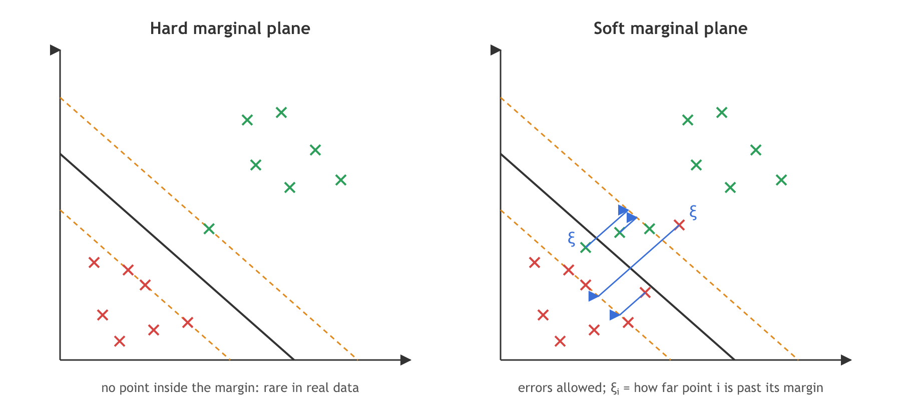
To work with lines in any number of dimensions, the video rewrites the line. y = mx + c and ax + by + c = 0 are the same line: solving the second for y gives y = −(a/b)x − c/b, so m = −a/b and the intercept is −c/b. With more features the line becomes y = w₁x₁ + w₂x₂ + … + b, written wᵀx + b.
Finding which side of the hyperplane a point is on
The video takes a line through the origin with slope −1, so b = 0. For the point (−4, 0), below the line, wᵀx + b comes out positive. For the point (4, 4), above the line, it comes out negative. So the sign of wᵀx + b tells the two classes apart: every point on one side gives a positive value and every point on the other side a negative one.
The board's w = [−1, 0] describes the vertical axis, not this line; the slope −1 line through the origin is x₁ + x₂ = 0, with w = [−1, −1], which gives +4 for (−4, 0) and −8 for (4, 4).
Checking the sign of wᵀx + b
import numpy as np

w = np.array([-1, -1])    # the line x1 + x2 = 0: slope -1 through the origin
b = 0
for point in ([-4, 0], [4, 4]):
    value = w @ np.array(point) + b
print(point, "->", value, "positive side" if value > 0 else "negative side")[-4, 0] -> 4 positive side [4, 4] -> -8 negative side
Deriving the margin 2 / ‖w‖
The hyperplane is wᵀx + b = 0. The two marginal planes through the nearest points are written wᵀx + b = +1 on one side and wᵀx + b = −1 on the other. The video notes that the right-hand side could be any +k and −k; papers use +1 and −1, and scaling w and b makes them so.
Take a point x₁ on the +1 plane and a point x₂ on the −1 plane, and subtract the two equations. b cancels and wᵀ(x₁ − x₂) = 2. Dividing both sides by the length of w, ‖w‖, leaves the distance between the planes. The aim is to make it as large as possible by changing w and b.
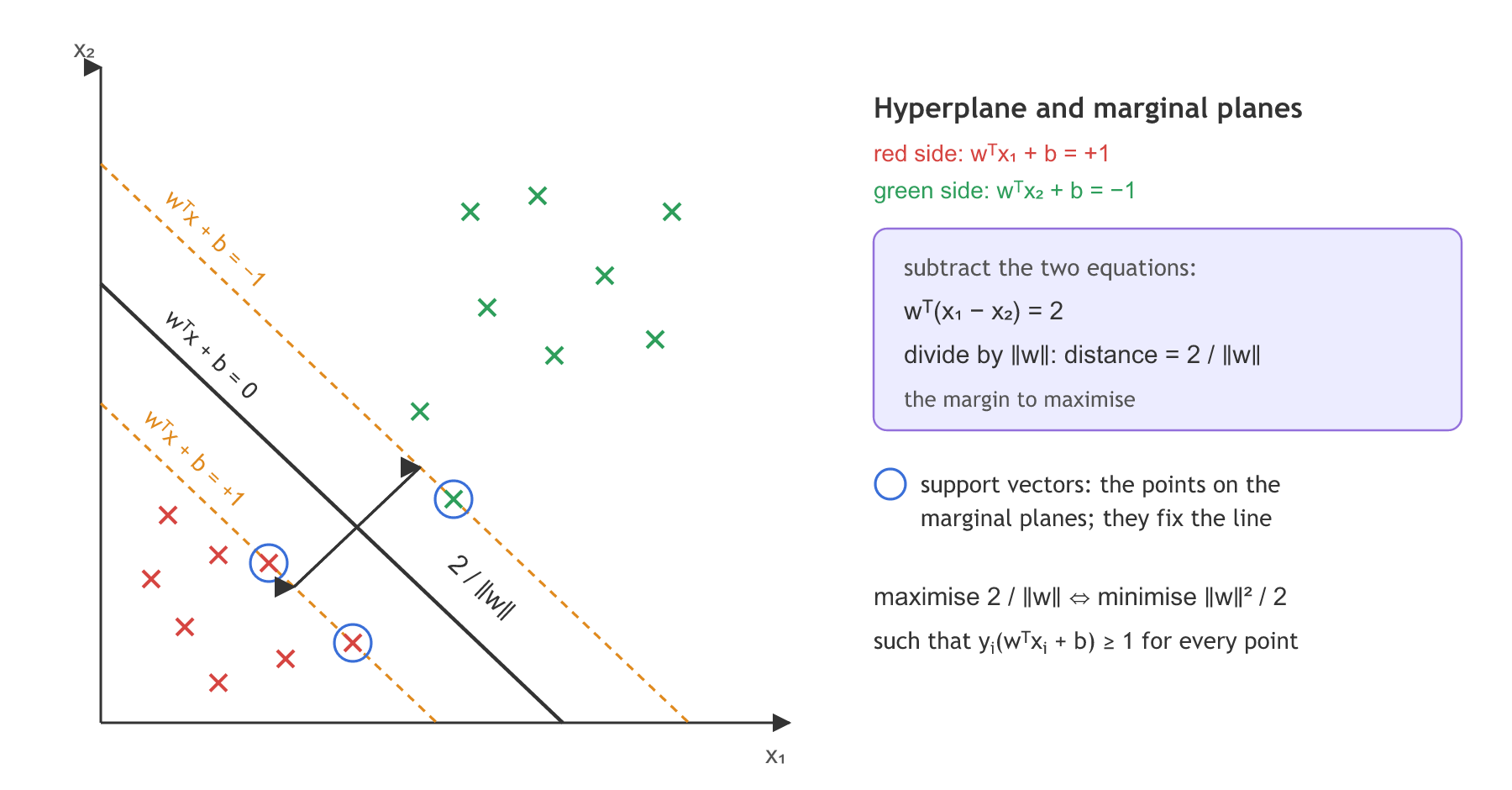
The points that lie on the marginal planes are the support vectors. They give the algorithm its name: move any other point a little and the hyperplane stays where it is.
Writing the optimisation with its constraint
Maximising the margin comes with a condition on every training point. A point of class +1 must have wᵀx + b ≥ 1, and a point of class −1 must have wᵀx + b ≤ −1. Both fit in one line: multiply by the label yᵢ, and every correct point gives yᵢ(wᵀxᵢ + b) ≥ 1, since minus times minus is plus.
Machine learning usually writes a cost to minimise, so maximising 2/‖w‖ becomes minimising its inverse. The board writes ‖w‖/2; the standard form is ‖w‖²/2, which has the same minimum and is smooth, so it is easier to optimise. The video says w and b are updated by back propagation. An SVM is not trained that way: the minimisation is a quadratic programming problem, and scikit-learn's SVC solves it with the libsvm solver.
Allowing errors with C and the slack ξ
For a soft marginal plane the cost gets a second term. For each point on the wrong side of its margin, ξᵢ (xi, the slack) is its distance past the margin, and the sum of these distances is added. C multiplies that sum.
The board describes C as how many errors the model can have, for example 6 or 7. C is one number for the whole model, and it is the price of each unit of error, not a count. A large C makes errors expensive, so the margin narrows to fit the training points; a small C makes them cheap, so the margin widens and more points are allowed inside it. The sum of the slacks is the hinge loss: each point's slack is ξᵢ = max(0, 1 − yᵢ(wᵀxᵢ + b)), which is 0 for every point on the right side of its margin and grows the farther a point is past it.
Changing the error term gives support vector regression (SVR), which the video leaves as an exercise: a tube of width ε around a regression line, with only the points outside the tube counted as errors. Support vector regression (SVR) works through it.
Separating curved data with a kernel
Some data cannot be split by a straight line, for example one class in a ring around the other. The video's answer is the SVM kernel: move the points from two dimensions into three, where one class rises and the other stays low, and split them there with a flat plane. SVM kernels shows how the kernels do it and compares them.
Fitting SVC on the board's points
A linear SVC with a very large C
kernel="linear" gives a straight hyperplane. A very large C makes every error so expensive that the fit behaves like a hard margin. After fitting, coef_ holds w, intercept_ holds b and support_vectors_ the points on the marginal planes.
from sklearn.svm import SVC

svm = SVC(kernel="linear", C=1000).fit(X, y)
w, b = svm.coef_[0], svm.intercept_[0]       # the hyperplane w^T x + b = 0
margin = 2 / np.linalg.norm(w) # the distance between the marginal planesimport numpy as np
from sklearn.svm import SVC
# The red points (+1) and green points (-1) of the margin drawing
X = np.array([[1, 1.2], [1.4, 2.1], [2.2, 0.8], [0.8, 2.6], [1.4, 0.5], [0.6, 1.8], [2, 2], [3, 1],
[4.6, 5.2], [5.4, 4.6], [6, 5.6], [4.4, 6.4], [6.6, 4.8], [5.2, 6.6], [6.8, 6.4],
[3.8, 3.9], [4.2, 2.8]])
y = np.array([1] * 8 + [-1] * 9)
svm = SVC(kernel="linear", C=1000).fit(X, y)
w, b = svm.coef_[0], svm.intercept_[0]
print("w:", w.round(3), " b:", round(b, 3))
print("support vectors:", svm.support_vectors_.tolist())
print("w^T x + b at the support vectors:", (svm.support_vectors_ @ w + b).round(3))
print("margin 2/||w||:", round(2 / np.linalg.norm(w), 3))w: [-0.667 -0.666] b: 3.667 support vectors: [[4.2, 2.8], [2.0, 2.0], [3.0, 1.0]] w^T x + b at the support vectors: [-1. 1. 1.] margin 2/||w||: 2.121
What the fitted hyperplane says
- w is about [−0.667, −0.666] and b about 3.667, so the hyperplane is the line x₁ + x₂ = 5.5, the solid line in the drawing.
- Three support vectors: (4.2, 2.8) on the green side and (2, 2), (3, 1) on the red side.
- wᵀx + b is −1 and +1 at them (up to rounding), so they sit on the marginal planes, and every other point is farther out.
- The margin is 2.121, which is the distance between the lines x₁ + x₂ = 4 and x₁ + x₂ = 7: 3 / √2.
Changing C on overlapping data
Two blobs from make_blobs with a large spread overlap, so a soft margin is needed. The same linear SVM runs with three values of C.
from sklearn.datasets import make_blobs

X, y = make_blobs(n_samples=200, centers=2, cluster_std=2.2, random_state=0)
for C in (0.01, 1, 100):
    m = SVC(kernel="linear", C=C).fit(X, y)
    print(f"C={C:<5} support vectors {m.n_support_.sum():3}   train accuracy {m.score(X, y):.3f}   "
f"margin {2 / np.linalg.norm(m.coef_):.2f}")C=0.01 support vectors 107 train accuracy 0.820 margin 4.49 C=1 support vectors 86 train accuracy 0.810 margin 3.29 C=100 support vectors 85 train accuracy 0.810 margin 3.25
What the three values of C did
- C = 0.01 makes errors cheap: the margin is wide (4.49) and 107 of the 200 points are support vectors, because every point inside the margin counts as one.
- C = 1 and C = 100 narrow the margin to 3.29 and 3.25 and use 86 and 85 support vectors.
- The training accuracy stays near 0.81 to 0.82: the blobs overlap, and no straight line separates them better. C changes the margin, not the shape of the boundary.
SVM vs logistic regression
| SVM | Logistic regression | |
|---|---|---|
| What it finds | the hyperplane with the widest margin | the line that maximises the likelihood |
| Points that shape it | only the support vectors | every training point |
| Output | a class (a probability needs extra calibration) | a probability through the sigmoid |
| Curved boundaries | kernels (rbf, polynomial) | only by adding features by hand |
| Scaling the features | needed, distances and margins depend on it | recommended for the solver |
Where you use support vector machines
- Text classification, such as spam filtering, where there are many features and a linear SVM does well.
- Small and medium datasets with a clear margin, such as image or gene expression data with a few thousand rows.
- Curved class boundaries, with the rbf kernel, when a linear model underfits.
StandardScaler in a Pipeline. A feature measured in thousands otherwise decides the margin alone. SVC training time also grows fast with the number of rows; for hundreds of thousands of rows use LinearSVC.Related
- Previous: XGBoost regressor
- Next: Support vector regression (SVR)
- See also: Logistic regression
- Reference: scikit-learn user guide, Support Vector Machines
- Remove the point [3, 1] from
X, change[1] * 8to[1] * 7iny, and refit: check which points stay support vectors and how the margin changes. - Change
C=1000toC=0.1on the board's points and print the support vectors again. - In the overlapping blobs, print
m.n_support_for C = 0.01 to see how many support vectors each class has.
You understood something today that you didn't yesterday.