Hierarchical clustering
Hierarchical clustering is an unsupervised learning algorithm that merges the nearest points and groups one step at a time into a tree called a dendrogram.
Last updated: 05 Oct, 2026 · scikit-learn 1.9.1
K-means clustering needs K before it starts. Hierarchical clustering builds every grouping, from one cluster per point up to a single cluster, and the dendrogram shows where to stop.
Merging P1 to P7 nearest first
The board places seven points, P1 to P7, and each point starts as its own cluster. The two nearest points, P1 and P2, merge first. Then P6 and P7 merge, then P3 and P5. P4 joins the group of P3 and P5, that group joins P1 and P2, and last of all P6 and P7 join the rest, leaving one cluster.
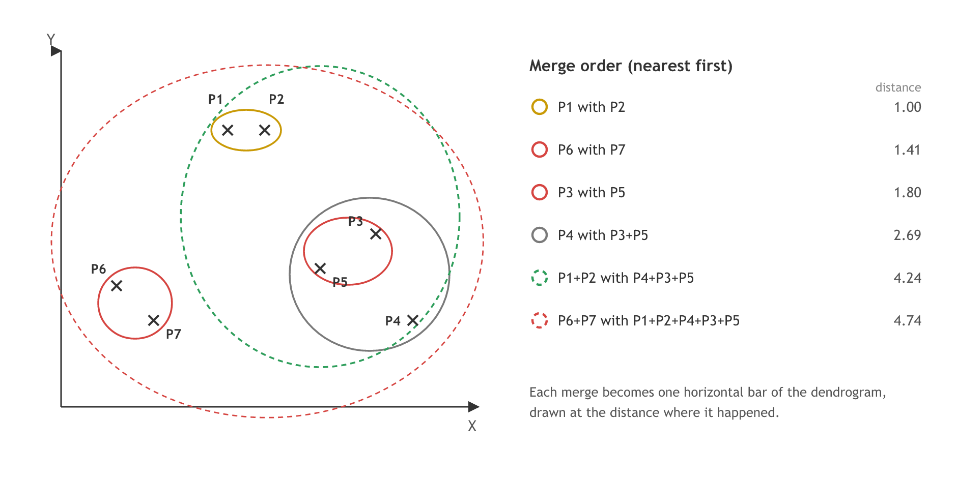
Once a group has several points, "nearest" needs a rule. The diagram and the code use single linkage: the distance between two groups is the distance between their two closest members, which is how the video describes the merges. The distances beside the diagram come from the run below.
Reading the dendrogram and cutting it
Each merge is drawn as a bar that joins two branches, at the height of the distance where the merge happened. Single points sit at the bottom and the last merge at the top. This tree is the dendrogram.
To choose the number of clusters, the board gives a rule: find the longest vertical line that no horizontal line passes through, and draw a horizontal cut across it. The number of vertical lines the cut crosses is the number of clusters. That longest line always sits in the biggest gap between two merge heights.
The board cuts at about 3 and counts 4 clusters, and in the next minute the video says the answer may be three, since the bars were drawn by eye. With the real distances in the run below, the biggest gap runs from 2.69 to 4.24, so the cut gives 3 clusters.
Agglomerative and divisive clustering
The board notes split hierarchical clustering into two kinds that build the same tree from opposite ends.
- Agglomerative works bottom up, the way the board merges P1 to P7: every point starts as its own cluster, the nearest two clusters merge, and the merging goes on until one cluster is left.
- Divisive works top down: all points start in one cluster, which is split again and again until every point stands alone.
The notes then read the cut as a threshold on the Euclidean distance. Every merge above the threshold is undone, so a higher threshold leaves fewer clusters. On the P1 to P7 tree, a threshold of 2.0 gives 4 clusters, 3.47 gives 3, and 4.5 gives 2.
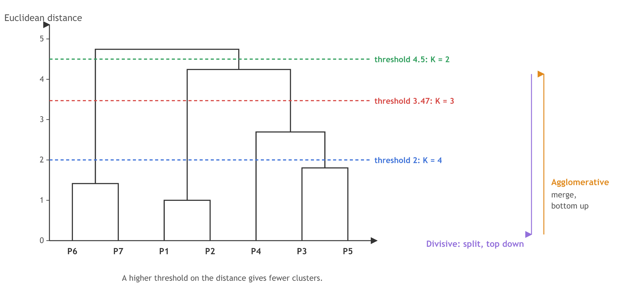
scikit-learn's AgglomerativeClustering, used below, is agglomerative. For the top-down direction scikit-learn has BisectingKMeans, which splits one cluster in two with K-means at each step.
Drawing the dendrogram with SciPy
The seven points and the linkage matrix
linkage() from SciPy runs every merge and returns one row per merge: the two clusters joined, the distance, and the size of the new cluster. Clusters 0 to 6 are the points; each merge creates the next number, 7, 8 and so on.
import numpy as np
from scipy.cluster.hierarchy import linkage

# P1 to P7, laid out like the board
points = np.array([[3, 9], [4, 9], [7, 6], [8, 3.5], [5.5, 5], [0, 4.5], [1, 3.5]])
names = ["P1", "P2", "P3", "P4", "P5", "P6", "P7"]

Z = linkage(points, method="single")   # nearest member to nearest member
print(Z.round(2))                      # one row per merge
Plotting the tree and the cut
from scipy.cluster.hierarchy import dendrogram
import matplotlib.pyplot as plt

dendrogram(Z, labels=names)
plt.axhline(y=3.47, color="red", linestyle="--")   # a cut inside the biggest gap
plt.show()
The P1 to P7 dendrogram from a real run
import numpy as np
import matplotlib.pyplot as plt
from scipy.cluster.hierarchy import linkage, dendrogram

points = np.array([[3, 9], [4, 9], [7, 6], [8, 3.5], [5.5, 5], [0, 4.5], [1, 3.5]])
names = ["P1", "P2", "P3", "P4", "P5", "P6", "P7"]
Z = linkage(points, method="single")

# Name every new cluster so the merges read like the board
groups = {i: [n] for i, n in enumerate(names)}
for k, (a, b, height, size) in enumerate(Z):
    groups[len(names) + k] = groups[int(a)] + groups[int(b)]
    print(f"{height:.2f}  {'+'.join(groups[int(a)])}  with  {'+'.join(groups[int(b)])}")

# The longest vertical line sits in the biggest gap between merge heights
gaps = np.diff(Z[:, 2])
cut = Z[gaps.argmax(), 2] + gaps.max() / 2
print("gaps:", gaps.round(2), " cut at", round(cut, 2))
print("clusters below the cut:", len(names) - (gaps.argmax() + 1))

dendrogram(Z, labels=names)
plt.axhline(y=cut, color="red", linestyle="--")
plt.title("Dendrogram")
plt.ylabel("Euclidean distance")
plt.show()1.00 P1 with P2 1.41 P6 with P7 1.80 P3 with P5 2.69 P4 with P3+P5 4.24 P1+P2 with P4+P3+P5 4.74 P6+P7 with P1+P2+P4+P3+P5 gaps: [0.41 0.39 0.89 1.55 0.5 ] cut at 3.47 clusters below the cut: 3
What the merges and the cut show
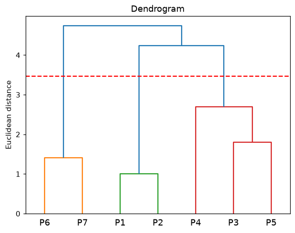
- The merge order is the board's: P1 with P2 (1.00), P6 with P7 (1.41), P3 with P5 (1.80), P4 with P3+P5 (2.69), P1+P2 with P4+P3+P5 (4.24), and P6+P7 with the rest (4.74).
- The biggest gap is 1.55, between 2.69 and 4.24, so the cut sits at 3.47.
- The cut crosses three vertical lines: {P1, P2}, {P3, P4, P5} and {P6, P7}.
Comparing single, complete, average and ward linkage
Single linkage is one of four common ways to measure the distance between two groups once they hold more than one point. Each one is a linkage method:
- Single: the two closest members, the formula above.
- Complete: the two farthest members.
- Average: the mean distance over every pair, one member from each group.
- Ward: merge the two groups whose union adds the least to the within-cluster sum of squares, the WCSS of the elbow method.
from scipy.cluster.hierarchy import linkage

for method in ["single", "complete", "average", "ward"]:
    Z = linkage(points, method=method)
    gaps = np.diff(Z[:, 2])                      # gaps between merge heights
    clusters = len(names) - (gaps.argmax() + 1)  # cut inside the biggest gap
print(f"{method:9} merge heights {Z[:, 2].round(2)} clusters: {clusters}")single merge heights [1. 1.41 1.8 2.69 4.24 4.74] clusters: 3 complete merge heights [1. 1.41 1.8 2.92 6.26 8.06] clusters: 3 average merge heights [1. 1.41 1.8 2.8 5.41 6.25] clusters: 3 ward merge heights [1. 1.41 1.8 3.07 8.25 9.47] clusters: 3
- The first three merges are the same for every method, at 1.00, 1.41 and 1.80. Each one joins two single points, and between two single points every method gives the plain distance.
- The later merges come out higher with complete, average and ward, because they look at more than the closest pair; ward climbs fastest, since joining two large groups adds a lot of squared distance. On these points every method still cuts into 3 clusters.
Getting the labels with AgglomerativeClustering
scikit-learn's AgglomerativeClustering runs the same merges and stops at n_clusters. Its default linkage is ward, which merges the two groups whose union adds the least within-group variance, so the code sets linkage="single" to match the board and prints ward next to it.
from sklearn.cluster import AgglomerativeClustering

single = AgglomerativeClustering(n_clusters=3, linkage="single").fit_predict(points)
print("single:", dict(zip(names, single.tolist())))

ward = AgglomerativeClustering(n_clusters=3).fit_predict(points)   # linkage="ward"
print("ward: ", dict(zip(names, ward.tolist())))single: {'P1': 2, 'P2': 2, 'P3': 0, 'P4': 0, 'P5': 0, 'P6': 1, 'P7': 1}
ward: {'P1': 2, 'P2': 2, 'P3': 0, 'P4': 0, 'P5': 0, 'P6': 1, 'P7': 1}- Single linkage gives the three groups of the cut: P1 and P2, P3 to P5, P6 and P7. The numbers 0, 1 and 2 are only names.
- Ward reaches the same three groups on these points. It joins them in a different order at the top: ward merges P1+P2 with P6+P7 before P3 to P5, so the full trees differ.
Cutting at a distance threshold
Instead of n_clusters, AgglomerativeClustering can take the threshold from the notes: set n_clusters=None and distance_threshold to the cut height, and it reports how many clusters that leaves in n_clusters_.
from sklearn.cluster import AgglomerativeClustering

for threshold in [2.0, 3.47, 4.5]:
    model = AgglomerativeClustering(n_clusters=None, distance_threshold=threshold,
                                    linkage="single").fit(points)
print(f"threshold {threshold}: {model.n_clusters_} clusters", model.labels_)threshold 2.0: 4 clusters [2 2 0 3 0 1 1] threshold 3.47: 3 clusters [2 2 0 0 0 1 1] threshold 4.5: 2 clusters [0 0 0 0 0 1 1]
The three thresholds give 4, 3 and 2 clusters, the counts the dendrogram above shows.
Clustering the Iris data with ward linkage
The hierarchical clustering notebook in the course materials runs on scikit-learn's Iris data: 150 flowers, 4 measurements each, and three species the clustering never sees. It scales the four features with StandardScaler, draws a ward dendrogram and fits AgglomerativeClustering with two clusters. Its fit line passes affinity='euclidean', and that line now fails:
import pandas as pd
from sklearn import datasets
from sklearn.preprocessing import StandardScaler
from sklearn.cluster import AgglomerativeClustering

iris = datasets.load_iris()
iris_data = pd.DataFrame(iris.data, columns=iris.feature_names)
X_scaled = StandardScaler().fit_transform(iris_data)

cluster = AgglomerativeClustering(n_clusters=2, affinity="euclidean", linkage="ward")Traceback (most recent call last):
File "main.py", line 10, in <module>
cluster = AgglomerativeClustering(n_clusters=2, affinity="euclidean", linkage="ward")
TypeError: AgglomerativeClustering.__init__() got an unexpected keyword argument 'affinity'scikit-learn renamed affinity to metric in version 1.2 and removed the old name in 1.4. With metric='euclidean' the notebook's model runs. The notebook also reduces the four features to two with PCA before clustering, so it can plot them; this run clusters the four scaled features directly. PCA has its own lesson, Principal component analysis (PCA).
import matplotlib.pyplot as plt
import scipy.cluster.hierarchy as sc

cluster = AgglomerativeClustering(n_clusters=2, metric="euclidean", linkage="ward")
cluster.fit(X_scaled)
print(pd.crosstab(cluster.labels_, iris.target_names[iris.target],
                  rownames=["cluster"], colnames=["species"]))

plt.figure(figsize=(12, 5))
sc.dendrogram(sc.linkage(X_scaled, method="ward"), no_labels=True)
plt.title("Dendrogram")
plt.xlabel("Sample Index")
plt.ylabel("Euclidean Distance")
plt.show()species setosa versicolor virginica cluster 0 1 50 50 1 49 0 0
What the Iris tree shows
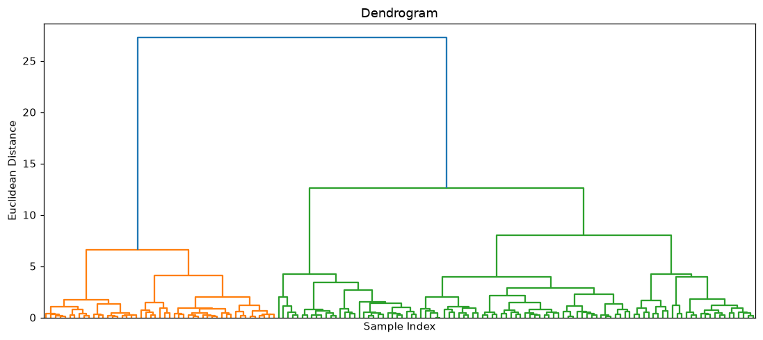
- Two clusters, as in the notebook: one holds 49 of the 50 setosa flowers, the other holds every versicolor and virginica flower plus one setosa.
- The longest vertical line sits under the top merge, so the board's rule also picks 2 clusters here, although there are three species. Versicolor and virginica overlap in their measurements; setosa stands apart.
- Checking the choice of 2 with a number is the job of the Silhouette score, which runs the notebook's silhouette loop on these clusters.
Comparing the time it takes on large data
The interview question from the video: which takes more time, K-means or hierarchical clustering? Hierarchical clustering. Every merge needs the distances between the current clusters, so the standard method works with every pair of points, n(n − 1)/2 of them. One K-means round only measures each point against K centroids. The video's advice: with a small dataset hierarchical clustering is fine; with a large one, use K-means.
# Distances each method has to work with, for n points and K = 4 clusters
for n in [1_000, 10_000, 100_000]:
    pairs = n * (n - 1) // 2      # every pair of points: hierarchical clustering
    per_round = n * 4             # every point to every centroid: one K-means round
print(f"n = {n:>7,}: {pairs:>13,} pairs vs {per_round:>7,} per K-means round")n = 1,000: 499,500 pairs vs 4,000 per K-means round n = 10,000: 49,995,000 pairs vs 40,000 per K-means round n = 100,000: 4,999,950,000 pairs vs 400,000 per K-means round
At 100,000 points there are almost 5 billion pairs against 400,000 distances per K-means round, and a dendrogram with 100,000 leaves cannot be read anyway.
Hierarchical clustering vs K-means
The board notes compare the two on scalability and flexibility: the size of the dataset, the kind of data each one handles, and how each one finds the number of clusters.
| Hierarchical clustering | K-means | |
|---|---|---|
| Number of clusters | chosen after, by cutting the dendrogram | K chosen before (elbow method) |
| Result | every grouping, from n clusters to 1 | one grouping with K clusters |
| Randomness | none: the same data gives the same tree | random starts (k-means++ helps) |
| Kind of data | any distance: Euclidean, Manhattan or cosine similarity (metric=) | numerical data, Euclidean distance to centroids |
| Dataset size | small | huge |
| Large data | slow: works with all pairs of points | fast: points against K centroids |
Where you use hierarchical clustering
- Small datasets where the tree itself helps: grouping a few hundred stores or products and reading which ones are closest.
- Biology: family trees of genes or species are dendrograms.
- Before K-means: cutting the tree on a sample gives a first guess for K.
Related
- Previous: K-means clustering
- Next: Silhouette score
- Reference: SciPy reference: dendrogram
- In the linkage comparison, add "centroid" to the list of methods and compare its merge heights with average linkage.
- Move P4 from [8, 3.5] to [8, 1] and run the dendrogram example again: does the cut still give 3 clusters?
- Set n_clusters=4 in the single-linkage AgglomerativeClustering and see which group splits.
Little by little, you're building something great.