Multiple linear regression
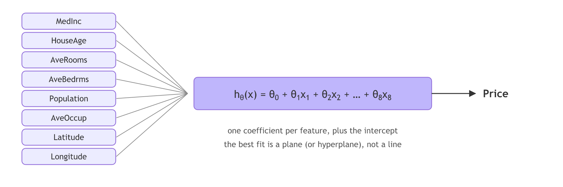
Multiple linear regression is a supervised learning algorithm that predicts a continuous output from two or more input features, fitting one coefficient per feature plus an intercept.
Last updated: 05 Oct, 2026 · scikit-learn 1.9.1
Real tables have many columns. The idea from Simple linear regression carries over unchanged: one θ per feature, the same cost function, and R² to score it.
The notes' example is a house pricing table: the number of rooms, the size of the house and its location predict the price, so hθ(x) = θ₀ + θ₁x₁ + θ₂x₂ + θ₃x₃, with θ₁, θ₂ and θ₃ the coefficients and θ₀ the intercept. The cost J(θ₀, θ₁, …) becomes a bowl over several parameters, and the best fit is a plane instead of a line.
Loading a housing dataset into a DataFrame
The video uses load_boston(), which scikit-learn removed in 1.2; the code here uses fetch_california_housing(). The steps are the same, the numbers are not.
The loader returns a Bunch, a dictionary-like object with key-value pairs: data holds the feature values, target the prices and feature_names the column names. The video combines them into a pandas DataFrame. Its first try sets the column names from target and gets an error:
import pandas as pd
from sklearn.datasets import fetch_california_housing

df = fetch_california_housing()   # downloads once, then reads from a local cache
dataset = pd.DataFrame(df.data)
dataset.columns = df.target # the video's first try: the wrong keyTraceback (most recent call last):
File "main.py", line 6, in <module>
dataset.columns = df.target # the video's first try: the wrong key
ValueError: Length mismatch: Expected axis has 8 elements, new values have 20640 elementsThe table has 8 columns and target holds 20,640 prices, one per row, so the lengths do not match. (Boston's message said 13 and 506.) The names live in feature_names.
Loading the table
import pandas as pd
from sklearn.datasets import fetch_california_housing

df = fetch_california_housing()   # downloads once, then reads from a local cache
dataset = pd.DataFrame(df.data)
Fixing the column names and adding Price
dataset.columns = df.feature_names   # 8 names for 8 columns
dataset["Price"] = df.target         # the output, as the last column
Adding the Price column and splitting X and y
The DataFrame so far holds only independent features. The video adds the dependent feature as a new column, Price, from target. Then it separates them: X takes every column except the last, and y takes the last column. In iloc[:, :-1] the part before the comma means all rows, and :-1 means every column but the last.
The video guesses that the Boston prices are in millions; they are in thousands of dollars. California's target is the median house value of a district, in units of 100,000 dollars.
Independent and dependent features
X = dataset.iloc[:, :-1]   # every column except the last: independent features
y = dataset.iloc[:, -1]    # the last column: the dependent feature
Splitting and fitting
from sklearn.model_selection import train_test_split
from sklearn.linear_model import LinearRegression

X_train, X_test, y_train, y_test = train_test_split(X, y, test_size=0.33, random_state=42)
lin_reg = LinearRegression()
lin_reg.fit(X_train, y_train)
Fitting California housing end to end
print(dataset.shape)
print(dataset.head(3).round(2).to_string())
print("intercept θ0:", round(lin_reg.intercept_, 2))
for name, theta in zip(X.columns, lin_reg.coef_):
print(f" {name:10} {theta:8.4f}")(20640, 9) MedInc HouseAge AveRooms AveBedrms Population AveOccup Latitude Longitude Price 0 8.33 41.0 6.98 1.02 322.0 2.56 37.88 -122.23 4.53 1 8.30 21.0 6.24 0.97 2401.0 2.11 37.86 -122.22 3.58 2 7.26 52.0 8.29 1.07 496.0 2.80 37.85 -122.24 3.52 intercept θ0: -37.08 MedInc 0.4449 HouseAge 0.0096 AveRooms -0.1220 AveBedrms 0.7791 Population -0.0000 AveOccup -0.0033 Latitude -0.4191 Longitude -0.4341
Scoring on the test set with r2_score
The video predicts on X_test, first with the lasso and ridge models from its practical (Ridge regression and Lasso regression), then with linear regression. That call first fails with "not fitted yet": the model was only passed to cross_val_score, which fits copies of it. Adding lin_reg.fit(X_train, y_train) fixes it. The score comes out at about 0.67 for Boston, and the video notes that a straight line limits how good it can get.
The video calls r2_score(y_pred, y_test) and says the order does not matter. The signature is r2_score(y_true, y_pred), and R² is not symmetric: the second line below shows the reversed call giving a different number.
from sklearn.metrics import r2_score

y_pred = lin_reg.predict(X_test)
print("r2_score(y_test, y_pred):", round(r2_score(y_test, y_pred), 4))
print("r2_score(y_pred, y_test):", round(r2_score(y_pred, y_test), 4), " <- reversed, as in the video")
print("lin_reg.score(X_test, y_test):", round(lin_reg.score(X_test, y_test), 4))r2_score(y_test, y_pred): 0.597 r2_score(y_pred, y_test): 0.3396 <- reversed, as in the video lin_reg.score(X_test, y_test): 0.597
Reading the coefficients and the score
- MedInc is +0.4449: one more unit of median income adds about 0.44 to the price, that is about 44,000 dollars, with the other features held fixed.
- AveBedrms is positive and AveRooms negative. The two are strongly related, so the model splits the credit between them; the signs do not say that bedrooms raise prices while rooms lower them.
- The test R² is 0.597: the plane explains about 60% of the variation in prices, the limit of a straight-line model the video mentions.
- The reversed call prints 0.3396, a different number for the same predictions.
lin_reg.scoregives the correct 0.597, since it always puts the true values first.
Predicting the index price from two rates
The practical notebook for this topic uses a smaller table, economic_index.csv: 24 months of the interest rate and the unemployment rate, and an index price to predict. With two features each coefficient is easy to read. The notebook drops the row number, year and month, splits with test_size=0.25, standardises, cross-validates and scores.
Loading and splitting the economic index
import pandas as pd
from sklearn.model_selection import train_test_split

url = ("https://raw.githubusercontent.com/krishnaik06/The-Grand-Complete-Data-Science-Materials/"
       "main/Machine%20Learning/2-Complete%20Linear%20Regression/Practicals/economic_index.csv")
df_index = pd.read_csv(url).drop(columns=["Unnamed: 0", "year", "month"])
X = df_index.iloc[:, :-1]   # interest_rate, unemployment_rate
y = df_index.iloc[:, -1]    # index_price
X_train, X_test, y_train, y_test = train_test_split(X, y, test_size=0.25, random_state=42)
Scaling and fitting
from sklearn.preprocessing import StandardScaler
from sklearn.linear_model import LinearRegression

scaler = StandardScaler()
X_train = scaler.fit_transform(X_train)
X_test = scaler.transform(X_test)   # the notebook calls fit_transform here
regression = LinearRegression().fit(X_train, y_train)
Scoring the index price model
import numpy as np
from sklearn.model_selection import cross_val_score
from sklearn.metrics import mean_squared_error, r2_score

print("coefficients:", regression.coef_.round(2), " intercept:", round(regression.intercept_, 2))
cv_mse = cross_val_score(LinearRegression(), X_train, y_train, scoring="neg_mean_squared_error", cv=3)
print("cross-validated MSE (cv=3):", round(-np.mean(cv_mse), 2))

y_pred = regression.predict(X_test)
score = r2_score(y_test, y_pred)
n, p = X_test.shape   # 6 test rows, 2 features
print("test MSE:", round(mean_squared_error(y_test, y_pred), 2))
print("test R²:", round(score, 4), " adjusted R²:", round(1 - (1 - score) * (n - 1) / (n - p - 1), 4))coefficients: [ 88.27 -116.26] intercept: 1053.44 cross-validated MSE (cv=3): 5914.83 test MSE: 5793.76 test R²: 0.8279 adjusted R²: 0.7132
Reading the index price model
- The coefficients are 88.27 and −116.26, as in the notebook: one standard deviation more interest rate adds about 88 to the index price, one more of unemployment takes about 116 off. The intercept, 1053.44, is the average training price.
- The cross-validated MSE is 5914.83, the notebook's −5914.83 without the minus sign of the "neg" scorer.
- The test R² is 0.8279 and adjusted R² 0.7132. The notebook prints 0.7591 and 0.5986, because it calls
scaler.fit_transform(X_test): the six test rows are scaled with their own mean and spread instead of the training rows', so the model sees them on a different scale. Fitting the scaler on the training rows only is the fix from Train and test split. - Adjusted R² is far below R² here because the test set is tiny: with n = 6 and p = 2 the penalty (n − 1) / (n − p − 1) is 5 / 3.
Boston in the video vs California here
| Boston (video) | California housing (here) | |
|---|---|---|
| Loader | load_boston(), removed in 1.2 | fetch_california_housing() |
| Rows and features | 506 rows, 13 features | 20,640 rows, 8 features |
| Target | Median value in 1000s of dollars | Median value in 100,000s of dollars |
| Test R² printed | About 0.67, with the arguments reversed | 0.597, with the arguments in order |
Where you use multiple linear regression
- Price and demand models with several drivers, such as house prices from income, age and location.
- Explaining a target: each coefficient is the change in the output for one unit of its feature, with the others held fixed.
- A baseline before Ridge regression, lasso and tree models.
Population prints about −0.0000 because one extra person in a district barely moves the price, not because population is unimportant. Scale the features first if you want to compare them.Related
- Previous: MSE, MAE and RMSE
- Next: Polynomial regression
- Reference: fetch_california_housing and LinearRegression
- Drop
LatitudeandLongitudefrom the California X withX.drop(columns=[...]), refit and compare the test R². - In the index price model, change
scaler.transform(X_test)toscaler.fit_transform(X_test): the test R² falls to 0.7591, the notebook's number. - Compute adjusted R² on the California test set with n =
len(X_test)and p = 8, using the function from R squared and adjusted R squared.
You understood something today that you didn't yesterday.