
Binomial distribution
The binomial distribution is the probability distribution of the number of successes in n independent trials that each have the same probability of success p.
Last updated: 07 Oct, 2026 · SciPy 1.18
The Bernoulli distribution describes one trial. Count the successes over many trials and you get the binomial distribution: heads in 10 tosses, defective items in a batch of 20, buyers among 100 visitors.
Counting successes in repeated trials
A count X has a binomial distribution, written X ~ B(n, p), when four conditions hold:
- A fixed number of trials n, decided in advance.
- Two outcomes per trial: success or failure, each trial a Bernoulli trial.
- Independent trials: one result does not change the others.
- The same p in every trial: a coin that changes from 0.5 to 0.6 halfway through does not give a binomial count.
The values are 0, 1, …, n. Each Bernoulli trial adds 0 or 1 to the count, so X is the sum of n independent Bernoulli variables with the same p.
Building the binomial PMF from three coin tosses
Toss a fair coin three times. There are 2 × 2 × 2 = 8 equally likely sequences. Exactly one head happens in 3 of them (HTT, THT, TTH), and 3 is C(3, 1), the number of ways to choose which toss is the head from Permutations and combinations.
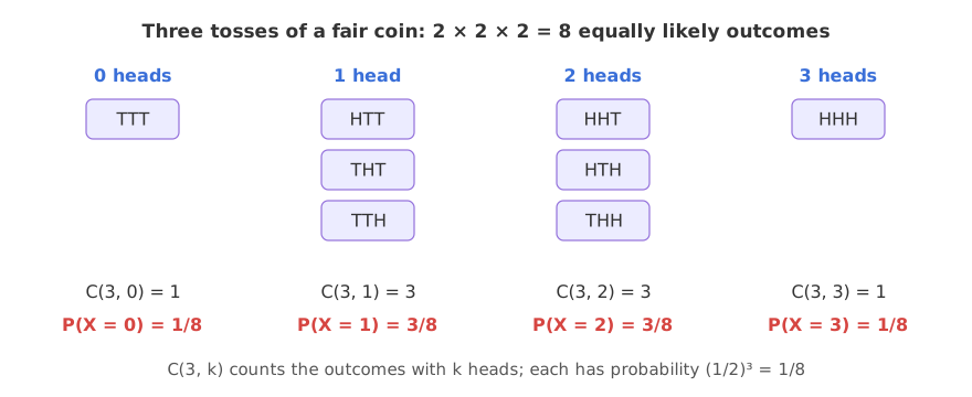
In general each sequence with k successes has probability pᵏ qⁿ⁻ᵏ, and there are C(n, k) such sequences:
The mean and variance are n times those of one Bernoulli trial, because X adds up n independent trials.
Working out P(X = 5) for ten tosses
Even the most likely count, 5 heads, happens in only about a quarter of runs of 10 tosses.
Computing binomial probabilities in scipy
stats.binom(n, p) gives the PMF, the CDF and the survival function sf(k) = P(X > k). The last lines rebuild the count as a sum of 10 Bernoulli trials and simulate it.
import numpy as np
from math import comb
from scipy import stats

print("C(10, 5) =", comb(10, 5), "  P(X = 5) =", round(comb(10, 5) * 0.5 ** 10, 4))
X = stats.binom(10, 0.5)
print("scipy: P(X = 5) =", round(X.pmf(5), 4), "  P(X <= 3) =", round(X.cdf(3), 4), "  P(X >= 8) =", round(X.sf(7), 4))
print("three tosses:", stats.binom(3, 0.5).pmf([0, 1, 2, 3]))
print("mean", X.mean(), " variance", X.var(), " (np and np(1 - p))")

for n, p in ((20, 0.5), (20, 0.7), (40, 0.5)):
    B = stats.binom(n, p)
    print(f"B({n}, {p}): mean {B.mean():.0f}  variance {B.var():.1f}  most likely count {np.argmax(B.pmf(np.arange(n + 1)))}")

rng = np.random.default_rng(42)
heads = (rng.random((100_000, 10)) < 0.5).sum(axis=1)   # 10 Bernoulli trials per row, added up
print("simulated P(X = 5):", round(np.mean(heads == 5), 4), " mean", round(heads.mean(), 3))C(10, 5) = 252 P(X = 5) = 0.2461 scipy: P(X = 5) = 0.2461 P(X <= 3) = 0.1719 P(X >= 8) = 0.0547 three tosses: [0.125 0.375 0.375 0.125] mean 5.0 variance 2.5 (np and np(1 - p)) B(20, 0.5): mean 10 variance 5.0 most likely count 10 B(20, 0.7): mean 14 variance 4.2 most likely count 14 B(40, 0.5): mean 20 variance 10.0 most likely count 20 simulated P(X = 5): 0.2473 mean 5.002
Plotting the binomial PMF
import numpy as np
import matplotlib.pyplot as plt
from scipy import stats

k = np.arange(0, 41)
plt.figure(figsize=(8, 4))
for n, p, c in ((20, 0.5, "tab:blue"), (20, 0.7, "tab:green"), (40, 0.5, "tab:red")):
    plt.plot(k, stats.binom.pmf(k, n, p), "o", color=c, label=f"n = {n}, p = {p}  (mean {n * p:.0f})")
    print(f"B({n}, {p}): tallest bar P(X = {n * p:.0f}) = {stats.binom.pmf(round(n * p), n, p):.4f}")
plt.title("Binomial PMF for three parameter sets")
plt.xlabel("k, number of successes")
plt.ylabel("P(X = k)")
plt.legend()
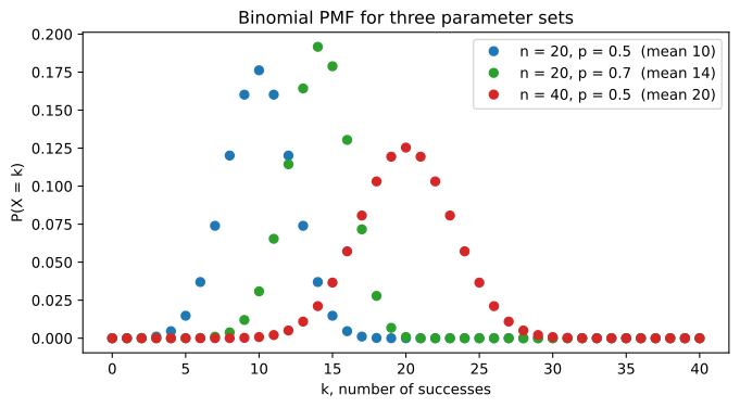
plt.show()B(20, 0.5): tallest bar P(X = 10) = 0.1762 B(20, 0.7): tallest bar P(X = 14) = 0.1916 B(40, 0.5): tallest bar P(X = 20) = 0.1254
What the binomial numbers show
- P(X = 5) = 0.2461 both by hand, 252 × 0.5¹⁰, and from scipy.
- P(X ≤ 3) = 0.1719 and P(X ≥ 8) = 0.0547: the two tails of ten fair tosses;
sf(7)is P(X > 7), the same as P(X ≥ 8). - Three tosses give 0.125, 0.375, 0.375 and 0.125, the 1/8, 3/8, 3/8, 1/8 of the diagram.
- The means are np: 10, 14 and 20 for the three parameter sets, with variances 5.0, 4.2 and 10.0. The most likely count sits at the mean here.
- Adding 10 Bernoulli trials reproduces the binomial: the simulated P(X = 5) is 0.2473, with a mean count of 5.002.
Binomial vs Poisson
| Binomial | Poisson | |
|---|---|---|
| Counts | Successes in n trials | Events in an interval of time or space |
| Largest value | n | No upper limit |
| Parameters | n and p | λ, the average count |
| Mean, variance | np, np(1 − p) | λ, λ |
| Link | Large n, small p | ≈ Poisson with λ = np |
Where you use the binomial distribution
- Quality control: the chance of more than 2 defective items in a batch of 20 when 5% of items are defective.
- Conversion counts: buyers among 1,000 visitors when each buys with probability 0.03.
- Testing a coin: in Hypothesis testing, the number of heads in 100 tosses of a fair coin is B(100, 0.5), which decides whether a result is unusual.
Related
- Previous: Bernoulli distribution
- Next: Poisson distribution
- Find P(X = 7) for
stats.binom(10, 0.7). Is it the most likely value? - A batch of 20 items has 5% defective. Compute P(more than 2 defective) with
stats.binom(20, 0.05).sf(2). - Check the mean and variance of
headsagainst np = 5 and np(1 − p) = 2.5 withheads.var().
Slow is fine. Stopping is the only problem.