
Bernoulli distribution
The Bernoulli distribution is the probability distribution of a single trial with two outcomes: success, coded 1, with probability p, and failure, coded 0, with probability q = 1 − p.
Last updated: 07 Oct, 2026 · SciPy 1.18
Random variables and probability distributions turned outcomes into numbers. The smallest such variable has two values, 0 and 1, and it is the building block of the binomial distribution in the next lesson.
Describing one coin toss with p and q
A Bernoulli trial has two outcomes, written 0 and 1, and only a single trial is involved. Two numbers describe it: p, the probability of the outcome coded 1, and q = 1 − p, the probability of the outcome coded 0.
- A fair coin: P(heads) = 0.5, so p = 0.5 and q = 1 − 0.5 = 0.5.
- An unfair coin: P(heads) = 0.3, so p = 0.3 and P(tails) = q = 1 − 0.3 = 0.7.
The distribution is named after the Swiss mathematician Jacob Bernoulli, and it is a discrete distribution. The video reads three examples off its Wikipedia figure: P(X = 0) = 0.2 with P(X = 1) = 0.8, the reverse 0.8 with 0.2, and 0.5 with 0.5.
Writing the Bernoulli PMF
Drawn as a chart, the distribution is two bars, one per outcome, whose heights add up to 1: 0.5 and 0.5 for the fair coin, 0.8 and 0.2 for a coin with P(heads) = 0.8. Because X takes separate values, this is a probability mass function, not a density. The PMF fits in one line:
The mean is p because E[X] = 0 × q + 1 × p. The variance p(1 − p) is largest, 0.25, for a fair coin, and shrinks towards 0 as the coin becomes more predictable. For the unfair coin with p = 0.3, Var(X) = 0.3 × 0.7 = 0.21.
Computing the Bernoulli distribution in scipy
import numpy as np
from scipy import stats

coin = stats.bernoulli(0.3)                 # the unfair coin: P(heads) = p = 0.3
print("P(X = 0) =", round(coin.pmf(0), 4), "  P(X = 1) =", round(coin.pmf(1), 4))
print("mean =", round(coin.mean(), 4), "  variance =", round(coin.var(), 4))

fair = stats.bernoulli(0.5)
print("fair coin: q =", round(fair.pmf(0), 4), "  mean =", fair.mean(), "  variance =", fair.var())

rng = np.random.default_rng(42)
heads = rng.random(10_000) < 0.3            # True counts as 1 (heads), False as 0
print("10,000 tosses: share of heads", heads.mean(), " variance", round(heads.var(), 4))P(X = 0) = 0.7 P(X = 1) = 0.3 mean = 0.3 variance = 0.21 fair coin: q = 0.5 mean = 0.5 variance = 0.25 10,000 tosses: share of heads 0.3043 variance 0.2117
Plotting the Bernoulli PMF for three coins
import matplotlib.pyplot as plt
from scipy import stats

fig, ax = plt.subplots(1, 3, figsize=(10, 3.4), sharey=True)
for a_, p in zip(ax, (0.5, 0.3, 0.8)):
    probs = stats.bernoulli(p).pmf([0, 1])
    a_.bar(["T (0)", "H (1)"], probs, width=0.5, color=["tab:green", "tab:red"])
    for k, v in enumerate(probs):
        a_.text(k, v + 0.02, f"{v:.1f}", ha="center")
    print(f"p = {p}: P(T) = {probs[0]:.1f}, P(H) = {probs[1]:.1f}")
    a_.set_title(f"p = {p}, q = {1 - p:.1f}")
ax[0].set_ylabel("Probability")
ax[0].set_ylim(0, 1)
fig.suptitle("Bernoulli PMF: one toss, two bars that add up to 1")
fig.tight_layout()
plt.show()p = 0.5: P(T) = 0.5, P(H) = 0.5 p = 0.3: P(T) = 0.7, P(H) = 0.3 p = 0.8: P(T) = 0.2, P(H) = 0.8
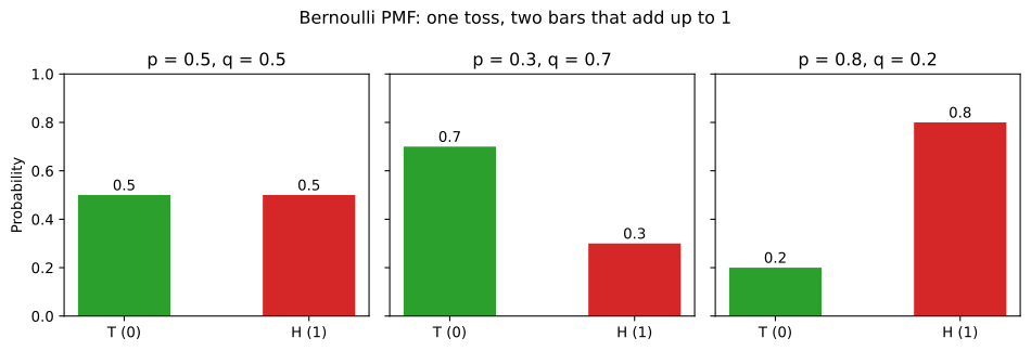
What the coin numbers show
- P(X = 0) = 0.7 and P(X = 1) = 0.3: q and p for the unfair coin.
- The mean is 0.3: the average of many 0s and 1s is the share of 1s, which is p.
- The variance is 0.21 = 0.3 × 0.7; the fair coin's 0.25 is the largest a Bernoulli variable can have.
- 10,000 simulated tosses give a share of 0.3043 and a variance of 0.2117, close to p and pq.
Bernoulli vs binomial
| Bernoulli | Binomial | |
|---|---|---|
| Trials | 1 | n independent trials, each with the same p |
| Values | 0 or 1 | 0, 1, …, n successes |
| Parameters | p | n and p |
| Mean, variance | p, p(1 − p) | np, np(1 − p) |
| scipy | stats.bernoulli(p) | stats.binom(n, p) |
Where you use the Bernoulli distribution
- Yes-or-no outcomes: a user clicks an ad or not, a payment is fraud or not, a patient responds or not.
- Binary classification: Logistic regression models each label as a Bernoulli variable whose p depends on the features.
- Proportions: the share of 1s in a sample is the mean of Bernoulli variables, which the z-test for a proportion builds on.
Related
- Change the coin to
stats.bernoulli(0.8). Are the mean 0.8 and the variance 0.16? - Print
stats.bernoulli(p).var()for p = 0.1, 0.3, 0.5, 0.7 and 0.9. Where is it largest? - Raise the simulation to 1,000,000 tosses. How much closer does the share of heads come to 0.3?
You understood something today that you didn't yesterday.