
Chi-square goodness-of-fit test
A chi-square goodness-of-fit test is a hypothesis test that checks whether the counts of one categorical variable match the counts expected from a stated set of proportions.
Last updated: 07 Oct, 2026 · SciPy 1.18
Means and t-tests need numbers. Many variables are categories: age bands, days of the week, product types. For those the data are counts, and the chi-square test compares the counts you see with the counts a claim predicts.
Defining the chi-square test
The video's definition: the chi-square test is about population proportions. It is a non-parametric test for categorical data, nominal or ordinal (see Measurement scales). Non-parametric here means it assumes no shape, normal or otherwise, for a numeric population: it works on the category counts alone. It treats the categories as unordered, so on ordinal data it does not use the order.
The video's interview advice: be able to say why a test fits a problem, not only how to compute it.
Setting up the census age problem
The problem on the board: in the 2000 Indian census, the ages of the individuals in a small town were found to be the following: under 18, 20%; 18 to 35, 30%; over 35, 50%. In 2010 the ages of n = 500 individuals were sampled, with these results: 121 under 18, 288 aged 18 to 35 and 91 over 35. Using α = 0.05, would you conclude that the population distribution of ages has changed in the last 10 years?
| < 18 | 18 to 35 | > 35 | |
|---|---|---|---|
| 2000 census share | 20% | 30% | 50% |
| 2010 sample count (n = 500) | 121 | 288 | 91 |
Computing the expected counts
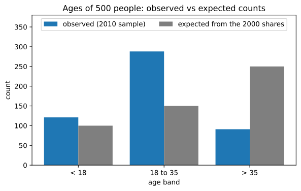
The test compares counts with counts, so the census shares become expected counts for a sample of 500: if the distribution had not changed, 500 × 0.20 = 100 people would be under 18, 500 × 0.30 = 150 would be 18 to 35 and 500 × 0.50 = 250 over 35. These sit next to the observed counts.
| < 18 | 18 to 35 | > 35 | Total | |
|---|---|---|---|---|
| Observed (2010) | 121 | 288 | 91 | 500 |
| Expected (500 × census share) | 100 | 150 | 250 | 500 |
The gaps are large: 138 more people aged 18 to 35 than expected and 159 fewer over 35. The test says whether gaps like these could come from sampling luck alone.
Stating the hypotheses and the decision rule
- ① Hypotheses: H₀: the 2010 ages follow the 2000 proportions, p₁ = 0.20, p₂ = 0.30, p₃ = 0.50. H₁: at least one proportion is different.
- ② Significance level: α = 0.05 (a 95% confidence level).
- ③ Degrees of freedom: df = k − 1, where k is the number of categories, not the sample size. With 3 age bands, df = 3 − 1 = 2.
- ④ Decision rule: the chi-square table at df 2 and α = 0.05 gives 5.991. Reject H₀ if χ² > 5.991.
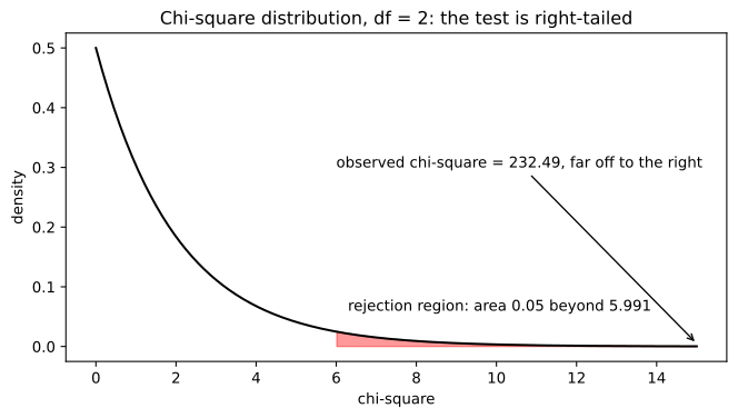
The chi-square goodness-of-fit test is right-tailed. Every gap between observed and expected, in either direction and in any cell, is squared and makes χ² larger, so only a large χ² counts against H₀. The whole α = 0.05 sits in the right tail, and 5.991 is the value with 0.05 of the area to its right, the area the chi-square table lists across its top.
Computing the chi-square statistic
232.494 > 5.991, so we reject H₀: the age distribution in 2010 is not the 2000 one. The p-value is about 3.3 × 10⁻⁵¹: if the 2000 shares still held, a sample of 500 this far from them would essentially never be drawn. The two big terms show where it changed: many more 18 to 35s (126.96) and far fewer over 35s (101.12).
Before trusting the χ² approximation check two conditions: the 500 people are independent of each other, and every expected count is at least 5. Here the smallest is 100.
Running the goodness-of-fit test in Python
Observed and expected counts
import numpy as np
from scipy import stats

observed = np.array([121, 288, 91])          # 2010 sample: <18, 18-35, >35
shares = np.array([0.20, 0.30, 0.50])        # 2000 census proportions
expected = observed.sum() * shares           # 500 x each share
The statistic, degrees of freedom and critical value
terms = (observed - expected) ** 2 / expected
chi2_stat = terms.sum()
df = len(observed) - 1                       # k - 1 categories
critical = stats.chi2.ppf(0.95, df) # right tail, alpha = 0.05print("expected:", expected)
print("terms (O - E)^2 / E:", terms.round(3))
print(f"chi-square = {chi2_stat:.3f}, df = {df}, critical = {critical:.3f}")
result = stats.chisquare(f_obs=observed, f_exp=expected)
print(f"scipy chisquare: statistic = {result.statistic:.3f}, p = {result.pvalue:.3g}")expected: [100. 150. 250.] terms (O - E)^2 / E: [ 4.41 126.96 101.124] chi-square = 232.494, df = 2, critical = 5.991 scipy chisquare: statistic = 232.494, p = 3.27e-51
import numpy as np
import matplotlib.pyplot as plt

bands = ["< 18", "18 to 35", "> 35"]
observed = [121, 288, 91]
expected = [100, 150, 250]
pos = np.arange(len(bands))
plt.figure(figsize=(7, 4))
plt.bar(pos - 0.2, observed, width=0.4, label="observed (2010 sample)", color="tab:blue")
plt.bar(pos + 0.2, expected, width=0.4, label="expected from the 2000 shares", color="tab:grey")
plt.xticks(pos, bands)
plt.ylim(0, 380)
plt.title("Ages of 500 people: observed vs expected counts")
plt.xlabel("age band")
plt.ylabel("count")
plt.legend(loc="upper center", ncol=2)
plt.show()
print("observed - expected:", np.array(observed) - np.array(expected))observed - expected: [ 21 138 -159]
import numpy as np
import matplotlib.pyplot as plt
from scipy import stats

x = np.linspace(0, 15, 400)
crit = stats.chi2.ppf(0.95, 2)
plt.figure(figsize=(8, 4))
plt.plot(x, stats.chi2.pdf(x, 2), color="black")
tail = x >= crit
plt.fill_between(x[tail], stats.chi2.pdf(x[tail], 2), color="red", alpha=0.4)
plt.text(crit + 0.3, 0.06, f"rejection region: area 0.05 beyond {crit:.3f}")
plt.annotate("observed chi-square = 232.49, far off to the right", xy=(15, 0.005), xytext=(6, 0.3),
             arrowprops=dict(arrowstyle="->"))
plt.title("Chi-square distribution, df = 2: the test is right-tailed")
plt.xlabel("chi-square")
plt.ylabel("density")
plt.show()
print("area to the right of the critical value:", round(stats.chi2.sf(crit, 2), 3))area to the right of the critical value: 0.05
Reading the chi-square output
- The expected counts print as 100, 150 and 250, the board's numbers.
- The three terms are 4.41, 126.96 and 101.124; their sum is the statistic.
- chi-square = 232.494 with df 2 against a critical value of 5.991: reject H₀.
- scipy's chisquare gives the same statistic and p = 3.27e-51. Its
ddofargument lowers the degrees of freedom when the expected shares were estimated from the same data; the census shares were not, so the default ddof = 0 keeps df = k − 1 = 2.
Testing equal shares: the school absences problem
A second problem from the notes that go with the video. A principal expects absences to be spread equally over the 5-day week. A sample of 100 absences gives Monday 23, Tuesday 16, Wednesday 14, Thursday 19 and Friday 28. With equal shares each expected count is 100/5 = 20, which is what chisquare assumes when no f_exp is given.
from scipy import stats

absences = [23, 16, 14, 19, 28]              # Mon to Fri, 100 absences
result = stats.chisquare(absences)           # f_exp defaults to equal counts: 20 each
print(f"chi-square = {result.statistic:.1f}, df = 4, p = {result.pvalue:.4f}")
print(f"critical value = {stats.chi2.ppf(0.95, 4):.3f}")
print("reject H0" if result.pvalue <= 0.05 else "fail to reject H0")chi-square = 6.3, df = 4, p = 0.1778 critical value = 9.488 fail to reject H0
χ² = 6.3 with df = 5 − 1 = 4 is below the critical 9.488, and p = 0.1778 > 0.05, so we fail to reject H₀. If absences were equally likely on every day, counts this uneven would turn up in about 18% of samples of 100. The data do not show a favourite day for being absent.
Goodness of fit vs test of independence
| Goodness of fit | Test of independence | |
|---|---|---|
| Variables | One categorical variable | Two categorical variables |
| Expected counts from | Stated proportions (the census shares) | Row total × column total / N |
| Degrees of freedom | k − 1 | (r − 1)(c − 1) |
| SciPy | chisquare(f_obs, f_exp) | chi2_contingency(table) |
Where you use a chi-square goodness-of-fit test
- Checking a sample against a population: does a survey's age or region mix match the census?
- Checking a fitted distribution: do counts per day follow the Poisson distribution fitted to them? (Then pass ddof = 1 for the estimated λ.)
- Fairness checks: does a die, a random number generator or a load balancer give each outcome its expected share?
chi2.ppf(0.95, df), not chi2.ppf(0.975, df), and df is the number of categories minus 1, not the sample size minus 1. It also needs counts, not percentages: 24.2% of 500 must become 121 before the test.Related
- Previous: Z-test for a proportion
- Next: Chi-square test of independence
- Reference: scipy.stats.chisquare
- Change the 2010 counts to 105, 160 and 235 (still 500 people). Is χ² now below 5.991?
- Pass the census shares as percentages,
f_exp=[20, 30, 50], and read the error SciPy raises. Why do the observed and expected totals have to match? - In the absences example change Friday to 38 and Monday to 13. Does the decision change?
This is what real progress feels like.