
Covariance
Covariance is a measure of how two numeric variables vary together: positive when they tend to rise and fall together, negative when one tends to fall as the other rises.
Last updated: 07 Oct, 2026 · SciPy 1.18
The tests so far compared groups. Often the question is about two measurements on the same things: do taller people weigh more, do students who study longer play less? Covariance is the first number that answers it.
Spotting how two variables move together
The video's first table pairs weight X with height Y for four people. As weight goes up, height goes up; as weight goes down, height goes down. Its second table pairs hours of study with hours of play: as study goes up, play goes down.
| Weight X (kg) | Height Y (cm) | Hours of study X | Hours of play Y | |
|---|---|---|---|---|
| 50 | 160 | 2 | 6 | |
| 60 | 170 | 3 | 4 | |
| 70 | 180 | 4 | 3 | |
| 75 | 181 |
Seeing the direction is easy with four rows. Covariance turns it into a number.
Computing covariance
For each pair, multiply how far x is from its mean by how far y is from its mean. The product is positive when both are above their means or both below, and negative when one is above and the other below. Covariance is the average of these products: divided by n for a whole population, and by n − 1 for a sample, as the board writes it, for the same reason as the Sample variance and why n − 1.
For the weight and height table, x̄ = 63.75 and ȳ = 172.75. The four products are 175.31, 10.31, 45.31 and 92.81, all positive, and they add up to 323.75:
Divided by n = 4 instead, the population covariance is 80.94. The study and play table gives −1.5: a negative covariance for a falling relationship. The notes that go with the video add a third small example, X = 2, 4, 6 and Y = 3, 5, 7, whose covariance is ((−2)(−2) + 0 + (2)(2))/2 = 4.
import numpy as np
import matplotlib.pyplot as plt

weight = np.array([50, 60, 70, 75])
height = np.array([160, 170, 180, 181])
sign = (weight - weight.mean()) * (height - height.mean())
plt.figure(figsize=(6, 4.5))
plt.axvline(weight.mean(), color="grey", linestyle="--")
plt.axhline(height.mean(), color="grey", linestyle="--")
plt.scatter(weight, height, s=80, c=np.where(sign > 0, "green", "red"))
for x, y, s in zip(weight, height, sign):
    plt.annotate(f"{s:+.1f}", (x, y), textcoords="offset points", xytext=(8, -12))
plt.xlim(45, 80)
plt.ylim(155, 185)
plt.title("Each point's (x - x̄)(y - ȳ): all four are positive")
plt.xlabel("weight (kg), dashed line at x̄ = 63.75")
plt.ylabel("height (cm), dashed line at ȳ = 172.75")
plt.show()
print("sum of products:", sign.sum(), " / (n - 1) =", round(sign.sum() / 3, 4))sum of products: 323.75 / (n - 1) = 107.9167
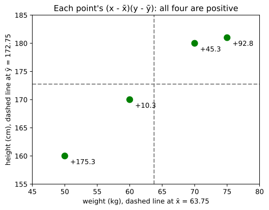
Reading the sign of covariance
- Positive: x and y tend to rise together and fall together (weight and height).
- Negative: when x rises, y tends to fall (study and play).
- Zero: no linear relationship. That is not the same as no relationship: points on a U-shape have a covariance near 0, because the products on the left and right halves cancel, even though y depends on x completely.
import numpy as np
import matplotlib.pyplot as plt

rng = np.random.default_rng(42)
x = rng.uniform(-3, 3, 200)
panels = {"rising": x + rng.normal(0, 0.8, 200),
          "falling": -x + rng.normal(0, 0.8, 200),
          "no pattern": rng.normal(0, 1.5, 200),
          "U-shape": x ** 2 + rng.normal(0, 0.5, 200)}
fig, axes = plt.subplots(1, 4, figsize=(13, 3.2))
for ax, (name, y) in zip(axes, panels.items()):
    c = np.cov(x, y)[0, 1]
    ax.scatter(x, y, s=8)
    ax.set_title(f"{name}: cov = {c:.2f}")
    ax.set_xlabel("x")
axes[0].set_ylabel("y")
plt.tight_layout()
plt.show()
print({name: round(float(np.cov(x, y)[0, 1]), 2) for name, y in panels.items()}){'rising': 3.12, 'falling': -2.81, 'no pattern': 0.14, 'U-shape': -0.21}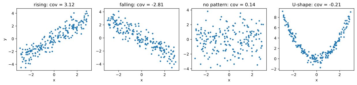
Computing covariance in Python
Deviation products by hand
import numpy as np

weight = np.array([50, 60, 70, 75])          # X
height = np.array([160, 170, 180, 181])      # Y
products = (weight - weight.mean()) * (height - height.mean())
Dividing by n − 1 or by n
cov_sample = products.sum() / (len(weight) - 1)    # divide by n - 1
cov_population = products.sum() / len(weight) # divide by nprint("deviation products:", products)
print("sample covariance:", round(cov_sample, 4), " population:", round(cov_population, 4))
print("np.cov:", np.cov(weight, height)) # 2 x 2 matrix, n - 1 by default
study, play = [2, 3, 4], [6, 4, 3]
print("study vs play:", np.cov(study, play)[0, 1])
print("X = 2, 4, 6 and Y = 3, 5, 7:", np.cov([2, 4, 6], [3, 5, 7])[0, 1])deviation products: [175.3125 10.3125 45.3125 92.8125] sample covariance: 107.9167 population: 80.9375 np.cov: [[122.91666667 107.91666667] [107.91666667 96.91666667]] study vs play: -1.5 X = 2, 4, 6 and Y = 3, 5, 7: 4.0
- The sample covariance is 107.9167 and the population covariance 80.9375.
- np.cov returns a 2 × 2 matrix. The off-diagonal entries are cov(weight, height) = 107.9167; the diagonal holds each variable's own sample variance, 122.9167 for weight and 96.9167 for height.
- Study vs play gives −1.5 and the notes' example gives 4.0, as worked above.
Why the size of a covariance is hard to read
Covariance carries the units of x times the units of y: kg·cm here. Measure height in metres instead of centimetres and the covariance shrinks 100 times, though the relationship is the same. So, as the video says, a covariance of +1000 is not "more related" than +100, and two covariances can only be compared when the units match. pandas shows it, and also shows that the covariance of a variable with itself is its variance:
import pandas as pd

df = pd.DataFrame({"weight_kg": [50, 60, 70, 75], "height_cm": [160, 170, 180, 181]})
df["height_m"] = df["height_cm"] / 100
print(df.cov().round(4))                     # pandas: ddof=1
print("var(weight) =", df["weight_kg"].var().round(4), "= cov(weight, weight)")weight_kg height_cm height_m weight_kg 122.9167 107.9167 1.0792 height_cm 107.9167 96.9167 0.9692 height_m 1.0792 0.9692 0.0097 var(weight) = 122.9167 = cov(weight, weight)
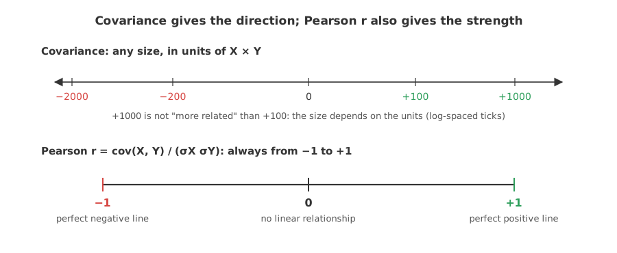
Dividing by the two standard deviations removes the units and fixes the range to −1 to +1. That is the Pearson correlation coefficient.
Covariance vs Pearson correlation
| Covariance | Pearson correlation r | |
|---|---|---|
| Formula | average of (x − x̄)(y − ȳ) | cov(x, y) / (s_x s_y) |
| Range | any value | −1 to +1 |
| Units | units of x × units of y | none |
| Tells you | the direction | the direction and the strength of a linear relationship |
| Weight and height table | 107.92 (n − 1) | 0.989 |
Where you use covariance
- Covariance matrices: Principal component analysis (PCA) finds the directions of largest variance from the covariance matrix of the features.
- Portfolio risk: the variance of a sum of returns adds twice the covariance of each pair, so assets with negative covariance reduce risk.
- Sums of variables: Var(X + Y) = Var(X) + Var(Y) + 2 cov(X, Y), so Var(X + Y) = Var(X) + Var(Y) only when the covariance is 0.
np.cov divides by n − 1 by default (bias=True gives n), while np.var divides by n by default (ddof=0). pandas .cov() and .var() both use n − 1. Mixing them gives a covariance matrix whose diagonal does not match your variances.Related
- Previous: Choosing a statistical test
- Next: Pearson correlation coefficient
- See also: Variance and standard deviation
- Reference: numpy.cov
- Add a fifth person, weight 80 kg and height 150 cm, to the arrays. Does the covariance stay positive?
- Run
np.cov(weight, height, bias=True). Is the off-diagonal entry 80.9375? - Change
height_mto height in millimetres (×10). How many times larger does its covariance with weight get?
Slow is fine. Stopping is the only problem.