
Poisson distribution
The Poisson distribution is the probability distribution of the number of events in a fixed interval of time or space, when the events happen independently at a constant average rate λ.
Last updated: 07 Oct, 2026 · SciPy 1.18
The Binomial distribution counts successes out of a fixed n. Many counts have no n: calls to a help desk in an hour, typos on a page, cars at a toll booth in a minute. The Poisson distribution models them with a single number, the average count λ (lambda).
Counting events in an interval
A count X follows a Poisson distribution, X ~ Poisson(λ), when events happen one at a time, independently of each other, at a steady average rate. The values are 0, 1, 2, … with no upper limit.
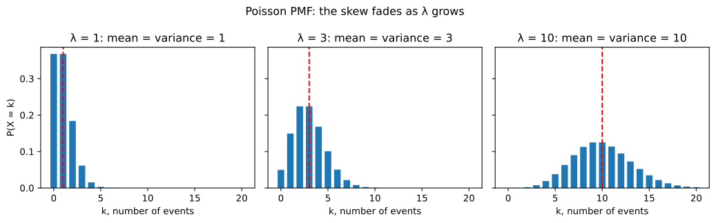
Its shape is skewed to the right for small λ, since counts cannot go below 0, and becomes more symmetric as λ grows. Its skewness is 1/√λ.
Working out help desk probabilities
A help desk gets 3 calls an hour on average, so λ = 3. The chance of a quiet hour with no calls is e⁻³ ≈ 0.0498. One call has probability 3e⁻³ ≈ 0.1494, and two and three calls are equally likely at about 0.2240 each.
Approximating the binomial with Poisson
When n is large and p small, the binomial B(n, p) is close to a Poisson with λ = np. Defects at a rate of 0.3% in a batch of 1,000 items, B(1000, 0.003), behave almost like Poisson(3).
Computing Poisson probabilities in scipy
from scipy import stats

calls = stats.poisson(3)                         # lambda = 3 calls per hour
for k in range(4):
    print(f"P(X = {k}) = {calls.pmf(k):.4f}")
print("P(X <= 2) =", round(calls.cdf(2), 4), "  P(X > 5) =", round(calls.sf(5), 4))
print("mean", calls.mean(), "  variance", calls.var(), "  skewness", round(float(calls.stats(moments="s")), 4))

B = stats.binom(1000, 0.003)                     # np = 3
print("binomial:", [round(float(B.pmf(k)), 4) for k in range(4)])
print("poisson: ", [round(float(calls.pmf(k)), 4) for k in range(4)])P(X = 0) = 0.0498 P(X = 1) = 0.1494 P(X = 2) = 0.2240 P(X = 3) = 0.2240 P(X <= 2) = 0.4232 P(X > 5) = 0.0839 mean 3.0 variance 3.0 skewness 0.5774 binomial: [0.0496, 0.1491, 0.2242, 0.2244] poisson: [0.0498, 0.1494, 0.224, 0.224]
Generating Poisson data like the video's notebook
The video's hypothesis-testing notebook makes up ages of students with stats.poisson.rvs, using seed 6. The loc argument shifts every value: loc=18, mu=35 draws a Poisson(35) count and adds 18, so the mean age is 18 + 35 = 53, not 35.
import numpy as np
import scipy.stats as stats

np.random.seed(6)
school_ages = stats.poisson.rvs(loc=18, mu=35, size=1500)
classA_ages = stats.poisson.rvs(loc=18, mu=30, size=60)
print("school mean:", school_ages.mean(), "  classA mean:", classA_ages.mean())
print("expected means:", stats.poisson(mu=35, loc=18).mean(), "and", stats.poisson(mu=30, loc=18).mean())
print("school variance:", round(school_ages.var(), 2), " (the shift does not change the variance, 35)")school mean: 53.303333333333335 classA mean: 46.9 expected means: 53.0 and 48.0 school variance: 36.98 (the shift does not change the variance, 35)
Plotting the Poisson PMF for three rates
import numpy as np
import matplotlib.pyplot as plt
from scipy import stats

k = np.arange(0, 21)
fig, ax = plt.subplots(1, 3, figsize=(11, 3.4), sharey=True)
for a_, lam in zip(ax, (1, 3, 10)):
    a_.bar(k, stats.poisson.pmf(k, lam), width=0.7)
    a_.axvline(lam, color="red", linestyle="--")
    a_.set_title(f"λ = {lam}: mean = variance = {lam}")
    print(f"lambda {lam}: P(X = {lam - 1}) = {stats.poisson.pmf(lam - 1, lam):.4f}, P(X = {lam}) = {stats.poisson.pmf(lam, lam):.4f}")
    a_.set_xlabel("k, number of events")
ax[0].set_ylabel("P(X = k)")
fig.suptitle("Poisson PMF: the skew fades as λ grows")
fig.tight_layout()
plt.show()lambda 1: P(X = 0) = 0.3679, P(X = 1) = 0.3679 lambda 3: P(X = 2) = 0.2240, P(X = 3) = 0.2240 lambda 10: P(X = 9) = 0.1251, P(X = 10) = 0.1251
What the Poisson numbers show
- P(0) = 0.0498, P(1) = 0.1494, P(2) = P(3) = 0.2240: the help desk's chances, from the PMF.
- P(X ≤ 2) = 0.4232 and P(X > 5) = 0.0839: fewer than three calls in about 42% of hours, more than five in about 8%.
- The mean and variance are both 3, and the skewness is 1/√3 = 0.5774.
- B(1000, 0.003) and Poisson(3) agree to within 0.0004 for 0 to 3 events: 0.0496 against 0.0498 for no events, 0.2244 against 0.2240 for three.
- The notebook's ages reproduce: a school mean of 53.3033 and a class A mean of 46.9, near the expected 53 and 48. The school ages have a variance of 36.98, close to the Poisson(35) variance of 35.
Poisson with a small vs a large λ
| λ = 1 | λ = 10 | |
|---|---|---|
| Most likely counts | 0 and 1 | 9 and 10 |
| Skewness 1/√λ | 1.0, clearly right-skewed | 0.32, close to symmetric |
| Normal approximation | Poor | Reasonable: N(10, 10) |
| Typical use | Rare events: failures per day | Busy counts: emails per hour |
Where you use the Poisson distribution
- Arrivals and traffic: customers per minute, requests to a server per second, calls per hour, used to size staff and servers.
- Rare events: defects per metre of cable, accidents per month at a junction.
- Counts in models: Poisson regression predicts counts such as the number of claims per policy.
Related
- Previous: Binomial distribution
- Next: Uniform distribution
- A page has 0.5 typos on average. Compute P(no typos) with
stats.poisson(0.5).pmf(0). - Compare
stats.binom(50, 0.06)withstats.poisson(3). Is the match worse than with n = 1000, p = 0.003? - Change the notebook's seed to 7. Does the school mean stay close to 53?
This is what real progress feels like.