
Power law and Pareto distribution
The Pareto distribution is a power-law probability distribution of positive values above a minimum x_m, in which a few very large values hold most of the total, as in the 80-20 rule.
Last updated: 07 Oct, 2026 · SciPy 1.18
The Log-normal distribution has a long right tail, but its tail still thins out quickly. Some quantities have heavier tails still: a few people hold most of the wealth, a few products make most of the sales. The Pareto distribution, a power law, describes them.
Reading the 80-20 rule
The video ties the power law to a rule to remember, the 80-20 rule: about 80% of the total comes from about 20% of the people or items. The examples are the video's own:
- 80% of the wealth is held by 20% of the people.
- 80% of a company's projects are done by 20% of the people in a team.
- 80% of sales come from the 20% most famous products.
- 80% of the oil comes from 20% of the land.
These are rules of thumb, known as the Pareto principle, not measurements; the real split varies from case to case. Data with this kind of distribution is said to follow a power law, and the Pareto distribution is the best-known power-law distribution.
Defining a power law and the Pareto distribution
A power law is a relationship y ∝ x⁻ᵏ: a relative change in x gives a proportional relative change in y, whatever the size of x. On log-log axes a power law is a straight line. The Pareto distribution has a power-law density above its minimum value x_m:
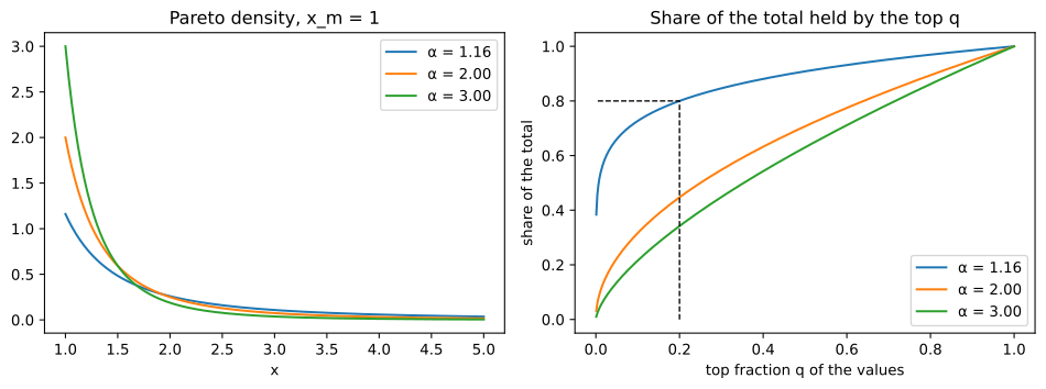
The shape parameter α (alpha) sets how heavy the tail is: the smaller α, the more of the total sits in the few largest values. The density is highest at x_m and falls from there, with no hump.
Finding the α behind 80-20
For a Pareto distribution with α > 1, the share of the total held by the top fraction q of values is q^(1 − 1/α). Setting the top 20% to hold 80% gives:
So only one Pareto distribution, α ≈ 1.161, gives exactly 80-20. With α = 2 the top 20% hold 44.7% of the total, and with α = 3 they hold 34.2%. Not every power law is an 80-20 split.
Computing the Pareto shares in Python
scipy's stats.pareto(b=α) is the Pareto distribution with x_m = 1 (use scale for another x_m). The code computes α, the share formula, and the share in one million simulated values.
import numpy as np
from scipy import stats

alpha_80_20 = np.log(5) / np.log(4)              # log base 4 of 5
print("alpha for 80-20:", round(alpha_80_20, 4))

for alpha in (alpha_80_20, 2, 3):
    formula = 0.2 ** (1 - 1 / alpha)             # share held by the top 20%
    x = np.sort(stats.pareto.rvs(b=alpha, size=1_000_000, random_state=42))
    simulated = x[-200_000:].sum() / x.sum()     # the largest 20% of the values
    print(f"alpha {alpha:.3f}: top 20% hold {formula:.3f} (formula), {simulated:.3f} (1,000,000 values)")

X = stats.pareto(b=2)
print("alpha 2: P(X > 10) =", X.sf(10), " mean", X.mean(), " variance", X.var())alpha for 80-20: 1.161 alpha 1.161: top 20% hold 0.800 (formula), 0.761 (1,000,000 values) alpha 2.000: top 20% hold 0.447 (formula), 0.447 (1,000,000 values) alpha 3.000: top 20% hold 0.342 (formula), 0.342 (1,000,000 values) alpha 2: P(X > 10) = 0.01 mean 2.0 variance inf
Plotting the Pareto density and the 80-20 curve
import numpy as np
import matplotlib.pyplot as plt
from scipy import stats

alphas = (np.log(5) / np.log(4), 2, 3)
fig, ax = plt.subplots(1, 2, figsize=(10, 3.8))
x = np.linspace(1, 5, 400)
for al in alphas:
    ax[0].plot(x, stats.pareto(b=al).pdf(x), label=f"α = {al:.2f}")
ax[0].set_title("Pareto density, x_m = 1")
ax[0].set_xlabel("x")
ax[0].legend()

q = np.linspace(0.001, 1, 400)                   # top share of the values
for al in alphas:
    ax[1].plot(q, q ** (1 - 1 / al), label=f"α = {al:.2f}")
ax[1].plot([0.2, 0.2, 0], [0, 0.8, 0.8], "k--", linewidth=1)
ax[1].set_title("Share of the total held by the top q")
ax[1].set_xlabel("top fraction q of the values")
ax[1].set_ylabel("share of the total")
ax[1].legend()
fig.tight_layout()
plt.show()
print("at q = 0.2:", [round(float(0.2 ** (1 - 1 / al)), 3) for al in alphas])at q = 0.2: [0.8, 0.447, 0.342]
What the Pareto shares show
- α = 1.161 gives exactly 80% for the top 20% by the formula; α = 2 gives 0.447 and α = 3 gives 0.342.
- The simulation matches for α = 2 and 3, at 0.447 and 0.342.
- For α = 1.161 one million values give only 0.761: the tail is so heavy that a sample rarely contains the extreme values that hold the rest. Heavy tails need very large samples.
- α = 2 has P(X > 10) = 0.01 and a mean of 2.0, but an infinite variance: for α ≤ 2 the variance does not exist, and for α ≤ 1 neither does the mean.
Telling Pareto apart from log-normal
Both are right-skewed and positive, but they are different distributions. The log-normal density has a hump and a tail that thins out faster than any power law; the Pareto density falls from x_m with no hump. Their logs differ too: the log of log-normal data is normal, while the log of Pareto data, ln(X/x_m), has an exponential distribution. On log-log axes the Pareto tail P(X > x) is a straight line and the log-normal tail bends down.
import numpy as np
import matplotlib.pyplot as plt
from scipy import stats

pareto = stats.pareto(b=1.5)
logn = stats.lognorm(s=1, scale=pareto.median())  # same median as the Pareto
x = np.logspace(0, 3, 200)

fig, ax = plt.subplots(1, 2, figsize=(10, 3.8))
ax[0].loglog(x, pareto.sf(x), label="Pareto α = 1.5")
ax[0].loglog(x, logn.sf(x), label="log-normal")
ax[0].set_title("Tail P(X > x) on log-log axes")
ax[0].set_xlabel("x")
ax[0].legend()
rng = np.random.default_rng(42)
ax[1].hist(np.log(pareto.rvs(size=50_000, random_state=rng)), bins=60, density=True, alpha=0.6, label="ln(Pareto)")
ax[1].hist(np.log(logn.rvs(size=50_000, random_state=rng)), bins=60, density=True, alpha=0.6, label="ln(log-normal)")
ax[1].set_title("After a log: exponential vs normal")
ax[1].legend()
fig.tight_layout()
plt.show()
print("median of each:", round(pareto.median(), 3), round(logn.median(), 3))
print("P(X > 100): Pareto", f"{pareto.sf(100):.1e}", "  log-normal", f"{logn.sf(100):.1e}")
print("P(X > 1000): Pareto", f"{pareto.sf(1000):.1e}", " log-normal", f"{logn.sf(1000):.1e}")median of each: 1.587 1.587 P(X > 100): Pareto 1.0e-03 log-normal 1.7e-05 P(X > 1000): Pareto 3.2e-05 log-normal 5.8e-11
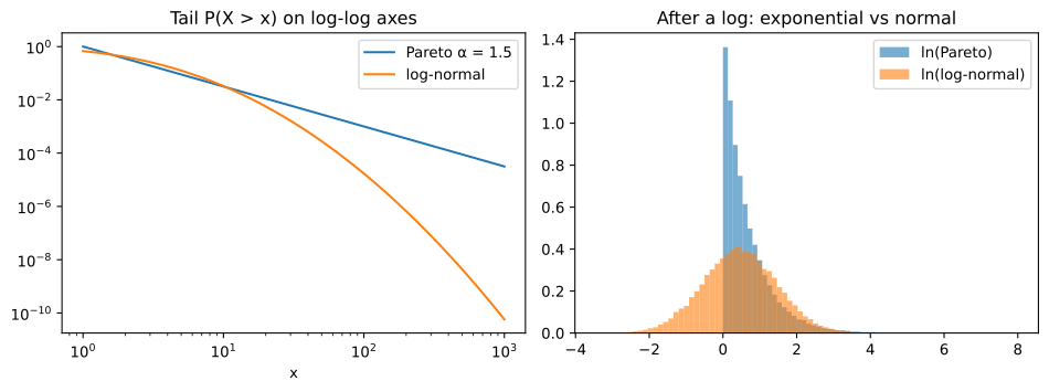
With the same median, 1.587, the Pareto distribution is nearly 60 times as likely to exceed 100 (1.0 × 10⁻³ against 1.7 × 10⁻⁵), and about 550,000 times as likely to exceed 1,000 (3.2 × 10⁻⁵ against 5.8 × 10⁻¹¹). That is what a heavy tail means.
Pareto vs log-normal
| Pareto | Log-normal | |
|---|---|---|
| Density shape | Highest at x_m, falls with no hump | Hump, then a long right tail |
| Tail on log-log axes | Straight line (power law) | Bends down |
| Log of the data | Exponential | Normal |
| Variance | Infinite when α ≤ 2 | Always finite |
| Typical data | Top wealth, city sizes, word frequencies | Most incomes, comment lengths |
Where you use the Pareto distribution
- Prioritising: finding the 20% of causes, customers or products that account for most of the effect.
- Risk: insurance claims and losses whose largest values dominate the total.
- Web and text data: page visits, followers and word frequencies, where a few items are huge.
Related
- Previous: Log-normal distribution
- Next: Central limit theorem
- Find the share held by the top 1% when α = 1.161:
0.01 ** (1 - 1 / 1.161). - Raise the simulation for α = 1.161 to 10,000,000 values. Does the simulated share move towards 0.8?
- Change the Pareto in the last example to
b=3. Does its line on the log-log plot get steeper?
You understood something today that you didn't yesterday.