
Probability density function (PDF) and KDE
A probability density function (PDF) is a function f(x) that describes how the probability of a continuous random variable is spread over its values: the area under f between a and b is the probability that the variable falls between a and b.
Last updated: 07 Oct, 2026 · SciPy 1.18
The video draws a smooth curve over the histogram of the 16 ages and calls it the PDF, made with a kernel density estimator. The curve is an estimate of a PDF from data. This lesson defines the PDF itself, its discrete partner the PMF and its running total the CDF, then builds the curve from the Histograms lesson with a KDE.
Describing a random variable
A random variable is a number whose value comes from a random process: the face a die shows, or the age of a student picked at random from the 16. Like the variables in Types of variables, it is discrete when it takes separate values and continuous when it can take any value in a range. Its distribution says how likely each value, or each range of values, is. The two kinds are described in different ways.
Listing probabilities with a PMF
A discrete random variable has a probability mass function (PMF): the probability of each value. A fair die has p(x) = 1/6 for each face 1 to 6. Every probability is between 0 and 1, and together they add up to 1.
Measuring probability as area under a PDF
A continuous random variable can take infinitely many values, so the probability of any one exact value is 0. The probability that a page takes exactly 2.700000 seconds to load is 0, while the probability that it takes between 2.5 and 3 seconds is a real number. A probability density function gives those range probabilities as areas:
The height f(x) is a density, probability per unit of x (per year, for ages), not a probability. It can even be larger than 1: a variable spread evenly between 0 and 0.5 has density 2 there, and 2 × 0.5 gives the total area of 1. The density histogram of the Histograms lesson is a rough PDF: its bars are drawn so their areas add up to 1.
Accumulating probability with the CDF
The cumulative distribution function (CDF) gives the probability of a value up to x. It works for both kinds of variable: for a die it is a staircase, for a continuous variable a smooth curve rising from 0 to 1. It turns any range into a subtraction, F(b) − F(a), and it is the cumulative relative frequency of the Frequency distribution lesson carried over to probabilities.
Computing the PMF and CDF of a die
from fractions import Fraction

pmf = {face: Fraction(1, 6) for face in range(1, 7)}
cdf = 0
for face, prob in pmf.items():
    cdf += prob
    print(f"P(X = {face}) = {prob}    F({face}) = P(X <= {face}) = {cdf}")
print("total probability:", sum(pmf.values()))
print("P(2 < X <= 5) = F(5) - F(2) =", Fraction(5, 6) - Fraction(1, 3))P(X = 1) = 1/6 F(1) = P(X <= 1) = 1/6 P(X = 2) = 1/6 F(2) = P(X <= 2) = 1/3 P(X = 3) = 1/6 F(3) = P(X <= 3) = 1/2 P(X = 4) = 1/6 F(4) = P(X <= 4) = 2/3 P(X = 5) = 1/6 F(5) = P(X <= 5) = 5/6 P(X = 6) = 1/6 F(6) = P(X <= 6) = 1 total probability: 1 P(2 < X <= 5) = F(5) - F(2) = 1/2
Estimating a PDF with kernel density estimation
Data never comes with its PDF; it has to be estimated. The video's idea is to smooth the histogram, and kernel density estimation (KDE) does that without bins. It places a small bell-shaped bump, the kernel, on every data point and averages the bumps. Where points crowd together the bumps pile up and the curve is high; where they are sparse it is low. Each bump has area 1/n, so the curve's total area is 1, as a PDF needs.
The bandwidth h is the width of each bump, and it plays the part the bin width plays in a histogram. Too small, and the curve has a spike at every point; too large, and real features such as a dip are smoothed away. SciPy's gaussian_kde picks it by Scott's rule: a factor of n−1/5 times the sample standard deviation. For the 16 ages the factor is 16−1/5 = 0.574.
Fitting a KDE to the ages
import numpy as np
from scipy.stats import gaussian_kde

ages = np.array([10, 12, 14, 18, 24, 26, 30, 35, 36, 37, 40, 41, 42, 43, 50, 51])
kde = gaussian_kde(ages)              # the bandwidth comes from Scott's rule by default
Measuring areas under the KDE of the ages
print("bandwidth factor :", round(kde.factor, 4))
print("kernel SD (years):", round(float(np.sqrt(kde.covariance[0, 0])), 2))
x = np.linspace(-20, 80, 2001)
density = kde(x)
print("highest density  :", round(float(density.max()), 4), "per year, at age", round(float(x[density.argmax()]), 1))
print("area under curve :", round(float(np.trapezoid(density, x)), 4))
print("P(20 <= age <= 40):", round(kde.integrate_box_1d(20, 40), 3))
print("share of the 16 ages in [20, 40]:", ((ages >= 20) & (ages <= 40)).mean())
print("P(age < 10) :", round(kde.integrate_box_1d(-np.inf, 10), 3))bandwidth factor : 0.5743 kernel SD (years): 7.57 highest density : 0.0265 per year, at age 38.5 area under curve : 1.0 P(20 <= age <= 40): 0.437 share of the 16 ages in [20, 40]: 0.4375 P(age < 10) : 0.087
Reading the KDE numbers
- Factor 0.5743 and kernel SD 7.57 years: Scott's rule makes each bump a bell about 7.6 years wide, 0.574 times the ages' standard deviation of 13.19.
- Highest density 0.0265 per year at about age 38.5: a density, not a probability. Over a 1-year stretch near 38.5 it means roughly a 2.6% chance.
- Area 1.0: the curve is a proper PDF.
- P(20 ≤ age ≤ 40) = 0.437 from the curve, close to the 7 of 16 ages (0.4375) that lie in that range: the area under the KDE tracks the share of the data.
- P(age < 10) = 0.087, though no age in the data is below 10: a KDE puts some probability beyond the smallest and largest values.
Drawing the KDE over the histogram
import matplotlib.pyplot as plt

x = np.linspace(-10, 75, 400)
fig, (ax1, ax2) = plt.subplots(1, 2, figsize=(11, 4))
ax1.hist(ages, bins=range(10, 70, 10), density=True, edgecolor="black", alpha=0.5,
         label="histogram, density=True")
ax1.plot(x, kde(x), color="red", label="KDE, Scott's rule")
ax1.set_title("Histogram and KDE of the ages")
ax1.set_xlabel("Age")
ax1.set_ylabel("Density")
ax1.set_ylim(0, 0.036)
ax1.legend(loc="upper left")
for bw, color in [(0.2, "orange"), ("scott", "red"), (1.0, "purple")]:
    ax2.plot(x, gaussian_kde(ages, bw_method=bw)(x), color=color, label=f"bw_method={bw}")
ax2.set_title("The bandwidth sets the smoothness")
ax2.set_xlabel("Age")
ax2.legend()
plt.show()
for bw in [0.2, "scott", 1.0]:
print(f"bw_method={bw}: peak density {gaussian_kde(ages, bw_method=bw)(x).max():.4f}")bw_method=0.2: peak density 0.0399 bw_method=scott: peak density 0.0265 bw_method=1.0: peak density 0.0209
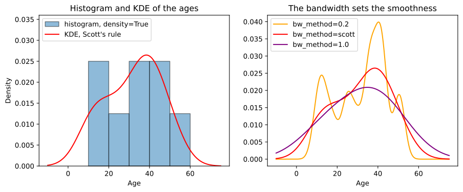
- On the density scale the bars are 0.025 and 0.0125 (4 or 2 ages ÷ 16 ÷ 10 years), and the red curve sits on the same scale, so the two can be compared.
- A factor of 0.2 gives bumps of about 2.6 years and a curve with several peaks; 1.0 gives one wide hill that hides the dip in the twenties. Their peaks are 0.0399, 0.0265 for Scott's rule, and 0.0209: a narrower bandwidth piles the same area of 1 into taller, thinner bumps.
PMF vs PDF vs CDF
| PMF | CDF | ||
|---|---|---|---|
| For | Discrete variables | Continuous variables | Both |
| Gives | P(X = x) | A density f(x); probability is an area | P(X ≤ x) |
| Range of values | 0 to 1, adding up to 1 | 0 or more, area 1 | Rises from 0 to 1 |
| Die / ages | 1/6 for each face | The KDE curve of the ages | 1/6, 1/3, ... 1; the area up to x |
| In SciPy | dist.pmf(x) | dist.pdf(x) | dist.cdf(x) |
Where you use PDFs and KDEs
- Exploring data:
sns.histplot(ages, stat="density", kde=True)orsns.kdeplotshows a column's shape without the jumps of a histogram. - Comparing groups: two KDE curves on one axis, such as bills at lunch and at dinner, overlap where the groups are alike.
- Named distributions: the normal distribution, in Normal (Gaussian) distribution, and the others in the later parts are PDFs and PMFs given by a formula, and SciPy's
pdf,pmfandcdfmethods compute them. A classifier such as Naive Bayes uses them to score each class.
integrate_box_1d or a CDF. Also remember that a KDE leaks past the data: here 8.7% of its area lies below age 10.Related
- Previous: Histograms
- Next: Mean, median and mode
- See also: Random variables and probability distributions
- Reference: SciPy gaussian_kde
- Compute
kde.integrate_box_1d(-np.inf, np.inf). Is the total area 1? - Fit
gaussian_kde(ages, bw_method="silverman")and print itsfactor. Is Silverman's rule wider or narrower than Scott's here? - Change the die to a loaded one, with face 6 at
Fraction(1, 2)and the other five atFraction(1, 10). Do the probabilities still add up to 1, and what is F(5)?
Every expert started right here.