
Pearson correlation coefficient
The Pearson correlation coefficient r is a measure of the strength and direction of the linear relationship between two numeric variables: their covariance divided by the product of their standard deviations, always between −1 and +1.
Last updated: 07 Oct, 2026 · SciPy 1.18
The Covariance of weight and height was 107.92, but on its own that number does not say whether the relationship is strong. Pearson's r rescales it to a fixed range, so any two correlations can be compared.
Scaling covariance into a correlation
The disadvantage of covariance, in the video's words: its magnitude has no limit. One pair of variables may give +100 and another +1000, and that says nothing about which pair is more related. Pearson's correlation coefficient fixes this by dividing by both standard deviations, which removes the units and restricts the value to −1 to +1.
The n − 1 in the covariance and in both standard deviations cancels, so r is the same whether you use the sample or the population formulas, as long as you use one of them throughout. The bound −1 ≤ r ≤ 1 is the Cauchy-Schwarz inequality.
For the weight and height table, s_x = 11.087 and s_y = 9.845, so r = 107.92 / (11.087 × 9.845) = 0.989: a strong positive linear relationship.
Reading values of r
- r = +1: every point lies on a rising straight line. r = −1: every point lies on a falling straight line.
- Between 0 and +1: a rising trend with scatter; the closer to +1, the tighter the points hug a line. Between −1 and 0: the same for a falling trend.
- r = 0: no linear relationship. As the video's examples show, curved patterns can have r = 0 even when y depends on x.
- The slope does not matter: a steep line and a shallow line both give r = 1. r measures how close the points are to a line, not how steep it is.
import numpy as np
import matplotlib.pyplot as plt

rng = np.random.default_rng(42)
targets = [1, 0.8, 0.4, 0, -0.4, -0.8, -1]
fig, axes = plt.subplots(1, 8, figsize=(16, 2.6))
x = rng.normal(size=300)
x = (x - x.mean()) / x.std()
noise = rng.normal(size=300)
noise = noise - noise.mean()
noise = noise - (noise @ x) / (x @ x) * x     # make the noise uncorrelated with x
noise = noise / noise.std()
for ax, rho in zip(axes, targets):
    y = rho * x + np.sqrt(1 - rho ** 2) * noise
    ax.scatter(x, y, s=4)
    ax.set_title(f"r = {round(np.corrcoef(x, y)[0, 1], 2) + 0.0:.2f}")
u = rng.uniform(-2, 2, 300)
axes[-1].scatter(u, u ** 2, s=4, color="tab:red")
axes[-1].set_title(f"U-shape: r = {np.corrcoef(u, u ** 2)[0, 1]:.2f}")
for ax in axes:
    ax.set_xticks([])
    ax.set_yticks([])
plt.tight_layout()
plt.show()
print("U-shape r:", round(np.corrcoef(u, u ** 2)[0, 1], 3))U-shape r: -0.056

Computing Pearson correlation in Python
r from the covariance
import numpy as np
from scipy import stats

weight = np.array([50, 60, 70, 75])
height = np.array([160, 170, 180, 181])
r_hand = np.cov(weight, height)[0, 1] / (weight.std(ddof=1) * height.std(ddof=1))res = stats.pearsonr(weight, height)
print("r by hand:", round(r_hand, 5), " np.corrcoef:", round(np.corrcoef(weight, height)[0, 1], 5))
print(f"pearsonr: r = {res.statistic:.5f}, p = {res.pvalue:.4f}")
print("study vs play r:", round(stats.pearsonr([2, 3, 4], [6, 4, 3]).statistic, 5))r by hand: 0.98874 np.corrcoef: 0.98874 pearsonr: r = 0.98874, p = 0.0113 study vs play r: -0.98198
- r = 0.98874 by hand, from
np.corrcoefand frompearsonr. - pearsonr also gives a p-value, here 0.0113, for H₀: ρ = 0 (no linear relationship in the population). If the true correlation were 0, four points would give an r at least this far from 0, in either direction, about 1% of the time. With only four points that test is weak, so read the p-value with care. The statistic behind it is t = r√(n − 2)/√(1 − r²) with n − 2 degrees of freedom.
- Study vs play gives r = −0.98198: a strong falling relationship.
A correlation matrix of a DataFrame
The video's notebook computes every pairwise correlation of the iris measurements with df.corr(). On pandas 2.0 and later that call fails, because the frame has a text column, species:
import seaborn as sns

df = sns.load_dataset("iris")
df.corr()Traceback (most recent call last):
File "main.py", line 4, in <module>
df.corr()
ValueError: could not convert string to float: 'setosa'pandas no longer drops non-numeric columns silently. Pass numeric_only=True:
import seaborn as sns

df = sns.load_dataset("iris")
print(df.corr(numeric_only=True).round(6))sepal_length sepal_width petal_length petal_width sepal_length 1.000000 -0.117570 0.871754 0.817941 sepal_width -0.117570 1.000000 -0.428440 -0.366126 petal_length 0.871754 -0.428440 1.000000 0.962865 petal_width 0.817941 -0.366126 0.962865 1.000000
import seaborn as sns
import matplotlib.pyplot as plt

df = sns.load_dataset("iris")
plt.figure(figsize=(6, 5))
sns.heatmap(df.corr(numeric_only=True), annot=True, fmt=".2f", cmap="coolwarm", vmin=-1, vmax=1)
plt.title("Pearson correlations of the iris measurements")
plt.show()
print("strongest pair: petal_length and petal_width,", round(df["petal_length"].corr(df["petal_width"]), 3))strongest pair: petal_length and petal_width, 0.963
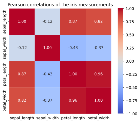
Sepal length and petal length have r = 0.871754, a strong positive correlation, as the video reads it. Petal length and petal width are the most related pair, 0.962865. Sepal width is weakly and negatively related to the others.
Correlation is not causation
A correlation says two variables move together in the data. It does not say one causes the other. The interview example: ice cream sales and drownings are positively correlated, because both rise in hot weather. Temperature is a lurking variable (a confounder) that drives both. To show cause you need an experiment, such as a randomized A/B test, or a careful causal analysis.
In Simple linear regression, r² is the share of the variance of y explained by the line: r = 0.989 gives r² = 0.978. See R squared and adjusted R squared.
Pearson r vs covariance
| Pearson r | Covariance | |
|---|---|---|
| Range | −1 to +1 | unbounded |
| Units | none, unchanged by rescaling | units of x × units of y |
| Compare across pairs | yes | only when the units match |
| Weight and height | 0.989 | 107.92 |
| Python | pearsonr, np.corrcoef, df.corr(numeric_only=True) | np.cov, df.cov() |
Where you use Pearson correlation
- Feature selection: the notes that go with the video drop one of two features that are 99% correlated, since they carry the same information. Use |r|: a correlation of −0.99 is as redundant as +0.99.
- Checking a linear model: a strong r between a feature and the target suggests a straight-line model can work.
- Multicollinearity: a correlation heatmap of the features shows pairs that make regression coefficients unstable.
Related
- Previous: Covariance
- Next: Spearman rank correlation
- Reference: scipy.stats.pearsonr
- Convert height to metres (
height / 100) and runpearsonragain. Does r change? - Add the point weight 120, height 150 to the arrays. How far does r fall?
- Print
df.corr(numeric_only=True, method="spearman")for iris and compare it with the Pearson matrix.
This is what real progress feels like.