
Sample variance and why n − 1
Sample variance is an estimate of a population's variance from a sample that divides the sum of squared deviations by n − 1 instead of n, so that on average it equals the true variance.
Last updated: 07 Oct, 2026 · SciPy 1.18
Variance and standard deviation wrote two formulas, one dividing by N and one by n − 1, and worked the six values 1, 2, 2, 3, 4, 5 both ways: 1.81 and 2.17. The n − 1 is called Bessel's correction, and the reason behind it is the number of degrees of freedom.
Measuring deviations from the sample mean
A sample is used to estimate the population variance σ², the average squared distance from the population mean μ. The sample does not know μ, so its deviations are taken from the sample mean x̄. The sample mean is computed from the same values, and it is the one number that makes their sum of squared deviations as small as possible. Any other centre, μ included, gives a larger sum:
So squared deviations from x̄ come out too small on average. Divided by n they give a variance that is too small by the factor (n − 1)/n. Dividing by n − 1 removes that bias: for independent draws, the expected value of s² is exactly σ².
Counting the degrees of freedom
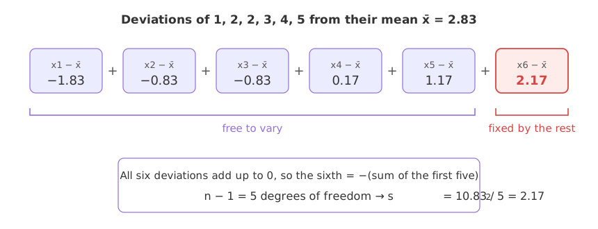
Deviations from the sample mean always add up to zero. For 1, 2, 2, 3, 4, 5 they are −1.83, −0.83, −0.83, 0.17, 1.17 and 2.17. Once the first five are known, the sixth is fixed: it has to bring the sum back to zero. Only n − 1 = 5 deviations are free to vary, so the sample carries n − 1 degrees of freedom for measuring spread, and the sum of squares is shared out over those five.
The same divisor appears whenever a mean is estimated from the data first: the covariance of x with itself is the sample variance, with n − 1 below it, and the t distribution of a one-sample t-test has n − 1 degrees of freedom.
Simulating the bias of dividing by n
A simulation shows the bias without algebra. Take the six values 1, 2, 2, 3, 4, 5 as a whole population, so its variance σ² = 1.806 is known. Draw a large number of samples of size n = 3 from it, with replacement so the draws are independent, compute each sample's variance both ways, and average each set of results. An unbiased estimate averages out to σ².
Drawing many samples at once
rng.choice with a two-number size returns a table: each row is one sample. It samples with replacement by default.
rng = np.random.default_rng(42)
samples = rng.choice(population, size=(200_000, 3))   # each row is a sample of n = 3
Both divisors on every sample
axis=1 computes one variance per row.
samples.var(axis=1, ddof=0)    # divides by n
samples.var(axis=1, ddof=1)    # divides by n - 1
Checking that the deviations add up to zero
import numpy as np

x = np.array([1, 2, 2, 3, 4, 5])
dev = x - x.mean()
print("deviations:", np.round(dev, 4))
print("sum of all six is zero:", np.isclose(dev.sum(), 0))
print("the sixth from the first five:", round(-dev[:5].sum(), 4))
print("sum of squares / 5:", round((dev ** 2).sum() / 5, 4), " np.var(ddof=1):", round(np.var(x, ddof=1), 4))deviations: [-1.8333 -0.8333 -0.8333 0.1667 1.1667 2.1667] sum of all six is zero: True the sixth from the first five: 2.1667 sum of squares / 5: 2.1667 np.var(ddof=1): 2.1667
Averaging 200,000 sample variances
import numpy as np

rng = np.random.default_rng(42)
population = np.array([1, 2, 2, 3, 4, 5])
sigma2 = population.var()                              # the true variance, divides by N
samples = rng.choice(population, size=(200_000, 3))    # 200,000 samples of n = 3

divide_n = samples.var(axis=1, ddof=0)
divide_n1 = samples.var(axis=1, ddof=1)
print("true variance:          ", round(sigma2, 4))
print("average of the ÷n:      ", round(divide_n.mean(), 4), "  (n-1)/n of the truth:", round(2 / 3 * sigma2, 4))
print("average of the ÷(n - 1):", round(divide_n1.mean(), 4))
print("true SD:", round(np.sqrt(sigma2), 4), " average sample SD:", round(np.sqrt(divide_n1).mean(), 4))true variance: 1.8056 average of the ÷n: 1.2031 (n-1)/n of the truth: 1.2037 average of the ÷(n - 1): 1.8047 true SD: 1.3437 average sample SD: 1.2102
What the simulation shows
- The deviations sum to zero, and the sixth one, 2.1667, is minus the sum of the other five.
- The ÷n estimates average 1.2031, two thirds of the true variance 1.8056, as the factor (n − 1)/n = 2/3 predicts.
- The ÷(n − 1) estimates average 1.8047, the true variance up to simulation noise.
- The sample standard deviation averages 1.2102, below the true 1.3437. Bessel's correction makes s² unbiased, but its square root s is still biased low.
Repeating the simulation for n from 2 to 10
import numpy as np
import matplotlib.pyplot as plt

rng = np.random.default_rng(42)
population = np.array([1, 2, 2, 3, 4, 5])
sigma2 = population.var()
sizes = range(2, 11)
avg_n, avg_n1 = [], []
for n in sizes:
    samples = rng.choice(population, size=(100_000, n))
    avg_n.append(samples.var(axis=1, ddof=0).mean())
    avg_n1.append(samples.var(axis=1, ddof=1).mean())
print("n:      ", list(sizes))
print("÷n:     ", np.round(avg_n, 3))
print("÷(n-1): ", np.round(avg_n1, 3))

plt.figure(figsize=(8, 3.6))
plt.axhline(sigma2, color="black", linestyle="--", label="true variance 1.806")
plt.plot(sizes, avg_n, "o-", color="red", label="average of ÷n")
plt.plot(sizes, avg_n1, "o-", color="blue", label="average of ÷(n - 1)")
plt.xlabel("sample size n")
plt.ylabel("average estimate")
plt.title("Dividing by n underestimates the variance")
plt.legend()
plt.show()n: [2, 3, 4, 5, 6, 7, 8, 9, 10] ÷n: [0.904 1.208 1.351 1.443 1.502 1.546 1.583 1.607 1.626] ÷(n-1): [1.807 1.812 1.801 1.803 1.803 1.804 1.809 1.808 1.807]
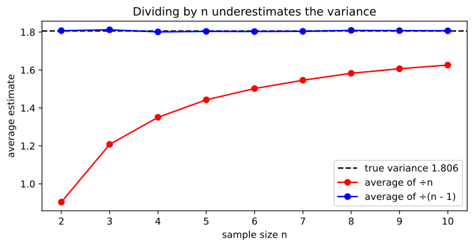
For n = 2 the ÷n estimate is half the truth, and the gap shrinks as n grows, because (n − 1)/n moves towards 1. For large samples the two divisors give almost the same number; for small ones the choice matters.
Population variance vs sample variance
| Population variance σ² | Sample variance s² | |
|---|---|---|
| Deviations from | the population mean μ | the sample mean x̄ |
| Divides by | N | n − 1 |
| Use it when | the data is the whole population | the data is a sample and σ² is unknown |
| NumPy | np.var(x) (ddof=0, default) | np.var(x, ddof=1) |
| pandas | s.var(ddof=0) | s.var() (ddof=1, default) |
Where you use the n − 1 divisor
- Survey and experiment data: any sample used to estimate the spread of a larger population.
- Standard errors and t-tests: the sample standard deviation s goes into s/√n (Point estimates and standard error).
- Not in feature scaling: scikit-learn's StandardScaler divides by the ÷n standard deviation, which makes little difference on large training sets.
np.var([5], ddof=1) returns nan with a warning. Small samples give unstable variance estimates even with the correction.Related
- Previous: Variance and standard deviation
- Next: Range, MAD and coefficient of variation
- See also: Point estimates and standard error
- Change
size=(200_000, 3)to(200_000, 6)and check that the ÷n average moves to 5/6 of 1.806. - Replace the population with
np.arange(1, 101)and check that the ÷(n − 1) average still lands on its variance,population.var(). - Run
np.var([5], ddof=1)and read the warning.
Slow is fine. Stopping is the only problem.