
P-value
The p-value is the probability, computed assuming the null hypothesis H₀ is true, of getting a test statistic at least as extreme as the one observed.
Last updated: 07 Oct, 2026 · SciPy 1.18
The Hypothesis testing lesson decided by checking whether the statistic fell beyond a critical value. The p-value reaches the same decision and also says how far into the tail the result sits.
Reading the p-value as a tail area
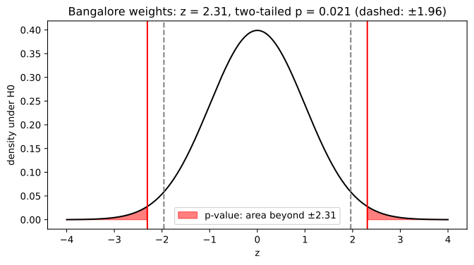
Start from the null distribution: the distribution the test statistic would have if H₀ were true. Mark the observed statistic on it. The p-value is the area of the tail (or both tails) beyond that mark, in the direction H₁ points:
- Small p: a result this extreme would be rare if H₀ were true, so the data are evidence against H₀.
- Large p: results like this are common under H₀, so the data give no reason to doubt it.
- Two-tailed test (H₁: μ ≠ μ₀): both tails count, so p = 2 × (area beyond |z|).
The p-value is not the probability that H₀ is true, not the probability that the result happened by chance, and not the share of the data falling in some region. It is a statement about the data, computed as if H₀ held.
Computing the p-value for the Bangalore weights
The Bangalore test gave z = (169.5 − 168)/(3.9/√36) = 2.31. A z-table gives Φ(z), the area to the left of z, not the area between −z and +z:
- Look up Φ(2.31): row 2.3, column 0.01, gives 0.98956.
- Upper tail: 1 − 0.98956 = 0.01044, the area to the right of 2.31.
- Both tails: H₁ is μ ≠ 168, so the lower tail below −2.31 counts too. By symmetry it is the same size: p = 2 × 0.0104 ≈ 0.021 (with the exact z = 2.3077, 2 × 0.01051 = 0.0210).
- Decide: 0.021 ≤ 0.05, so reject H₀ at α = 0.05, the same decision as the critical-value method.
Interpretation in the question's words: if the mean weight of all Bangalore residents were 168 pounds, a sample of 36 people with a mean at least 1.5 pounds away from 168, in either direction, would turn up about 2.1% of the time. That is rare enough to reject H₀ at the 5% level, but not at the 1% level, because 0.021 > 0.01.
Computing the Bangalore p-value in Python
norm.cdf(z) is the z-table, Φ(z). norm.sf(z) is the upper tail 1 − Φ(z), computed without the rounding loss of the subtraction. The last line computes the 95% confidence interval x̄ ± 1.96 × 0.65 for comparison.
import math
from scipy.stats import norm

z = (169.5 - 168) / (3.9 / math.sqrt(36))
print("z =", round(z, 4))
print("z-table row 2.3:", [round(float(norm.cdf(2.3 + c / 100)), 5) for c in range(10)])
print("Phi(2.31) =", round(norm.cdf(2.31), 5), "  upper tail 1 - Phi(2.31) =", round(1 - norm.cdf(2.31), 5))

p = 2 * norm.sf(abs(z))              # two-tailed: both tails beyond |z|
print("exact upper tail =", round(norm.sf(z), 5), "  two-tailed p =", round(p, 4))
for alpha in (0.05, 0.01):
    print(f"alpha = {alpha}:", "reject H0" if p <= alpha else "fail to reject H0")

lo, hi = 169.5 - 1.96 * 0.65, 169.5 + 1.96 * 0.65
print("95% CI:", round(lo, 2), "to", round(hi, 2), " contains 168:", lo <= 168 <= hi)z = 2.3077 z-table row 2.3: [0.98928, 0.98956, 0.98983, 0.9901, 0.99036, 0.99061, 0.99086, 0.99111, 0.99134, 0.99158] Phi(2.31) = 0.98956 upper tail 1 - Phi(2.31) = 0.01044 exact upper tail = 0.01051 two-tailed p = 0.021 alpha = 0.05: reject H0 alpha = 0.01: fail to reject H0 95% CI: 168.23 to 170.77 contains 168: False
What the Bangalore numbers show
- Row 2.3 of the z-table runs from 0.98928 (z = 2.30) to 0.99158 (z = 2.39); the cell for 2.31 is 0.98956.
- The two-tailed p is 0.021: twice the upper tail of 0.01051.
- p ≤ 0.05 rejects H₀, p > 0.01 does not: the same data can be significant at one level and not at a stricter one, which is why α must be chosen first.
- The 95% CI is 168.23 to 170.77 and excludes 168. A two-sided test at α rejects H₀: μ = μ₀ exactly when μ₀ lies outside the (1 − α) confidence interval, so the test and the interval agree.
import numpy as np
import matplotlib.pyplot as plt
from scipy.stats import norm

z = 2.3077
x = np.linspace(-4, 4, 500)
y = norm.pdf(x)
plt.figure(figsize=(8, 4))
plt.plot(x, y, color="black")
plt.fill_between(x, y, where=np.abs(x) >= z, color="red", alpha=0.5, label="p-value: area beyond ±2.31")
for c in (-1.96, 1.96):
    plt.axvline(c, color="grey", linestyle="--")
for v in (-z, z):
    plt.axvline(v, color="red")
plt.title("Bangalore weights: z = 2.31, two-tailed p = 0.021 (dashed: ±1.96)")
plt.xlabel("z")
plt.ylabel("density under H0")
plt.legend()
plt.show()
print("each tail:", round(norm.sf(z), 4), " both:", round(2 * norm.sf(z), 4))each tail: 0.0105 both: 0.021
Deciding with p ≤ α
The decision rule compares the p-value with the significance level α chosen before the data:
- p ≤ α: reject H₀.
- p > α: fail to reject H₀.
This is the same rule as the critical value: the statistic falls beyond the critical value exactly when its tail area is smaller than α. The p-value adds information the yes-or-no decision hides: 0.049 and 0.0001 both reject at 0.05, but the second is far stronger evidence.
Computing p-values for the fair coin
For the coin, binomtest computes the exact two-sided p-value from the binomial distribution: the probability, for a fair coin, of a head count at least as unlikely as the one observed.
from scipy.stats import binomtest

for x in (10, 25, 30, 50, 60, 95):
    p = binomtest(x, n=100, p=0.5).pvalue      # exact two-sided p-value
    verdict = "reject H0" if p <= 0.05 else "fail to reject H0"
print(f"{x:2} heads: p = {p:.3g} -> {verdict} at alpha 0.05")10 heads: p = 3.06e-17 -> reject H0 at alpha 0.05 25 heads: p = 5.64e-07 -> reject H0 at alpha 0.05 30 heads: p = 7.85e-05 -> reject H0 at alpha 0.05 50 heads: p = 1 -> fail to reject H0 at alpha 0.05 60 heads: p = 0.0569 -> fail to reject H0 at alpha 0.05 95 heads: p = 1.25e-22 -> reject H0 at alpha 0.05
- 30 heads: p = 7.85 × 10⁻⁵. A fair coin gives a result this lopsided less than once in 10,000 runs of 100 tosses, so H₀ is rejected.
- 50 heads: p = 1. Nothing is more typical of a fair coin. This does not mean H₀ is certainly true; it means the data contain no evidence against it.
- 60 heads: p = 0.0569, slightly above 0.05: fail to reject, but close. Report the p-value itself rather than only the verdict.
Separating evidence from effect size
A p-value measures evidence against H₀, not the size of an effect. The same 0.3-pound difference from 168 gives a very different p-value at two sample sizes:
import math
from scipy.stats import norm

# the same 0.3-pound difference from 168, with sigma 3.9, at two sample sizes
for n in (36, 3600):
    z = 0.3 / (3.9 / math.sqrt(n))
print(f"n = {n:4}: sample mean 168.3, z = {z:.2f}, two-tailed p = {2 * norm.sf(z):.2g}")n = 36: sample mean 168.3, z = 0.46, two-tailed p = 0.64 n = 3600: sample mean 168.3, z = 4.62, two-tailed p = 3.9e-06
With 36 people a 0.3-pound difference is well within chance (p = 0.64); with 3,600 people the same difference is overwhelming evidence (z = 4.62, p ≈ 3.9 × 10⁻⁶), yet 0.3 pounds may not matter to anyone. Always report the effect (the difference, or a confidence interval for it) next to the p-value.
P-value vs significance level α
| P-value | Significance level α | |
|---|---|---|
| What it is | Tail probability of the observed result under H₀ | Type I error rate the analyst accepts |
| When it is set | Computed from the data | Chosen before the data |
| Changes with the sample | Yes | No |
| Bangalore example | 0.021 | 0.05 |
| Rule | Reject H₀ when p ≤ α | Reject H₀ when p ≤ α |
Where you use p-values
- Every SciPy test (
ttest_1samp,ttest_ind,chi2_contingency,binomtest) returns a p-value to compare with α. - Regression output: statsmodels prints a p-value for each coefficient, testing H₀: coefficient = 0.
- A/B tests: the p-value for the difference in conversion rates, reported with the size of the difference.
Related
- Previous: Hypothesis testing
- Next: Significance level, one-tailed and two-tailed tests
- Reference: scipy.stats.norm
- Compute the p-value for the video's second problem: average age 24, σ = 1.5, a sample of 36 with mean 25. Is z = 4 and p about 6.3 × 10⁻⁵?
- Change the Bangalore sample mean to 169.0. Is the new p above or below 0.05?
- Run
binomtest(61, n=100, p=0.5).pvalue. Which side of 0.05 does 61 heads land on?
You understood something today that you didn't yesterday.