
One-sample t-test and the t distribution
A one-sample t-test is a hypothesis test that checks whether a population mean equals a stated value μ₀ when the population standard deviation is unknown, using the sample standard deviation s and the t distribution with n − 1 degrees of freedom.
Last updated: 07 Oct, 2026 · SciPy 1.18
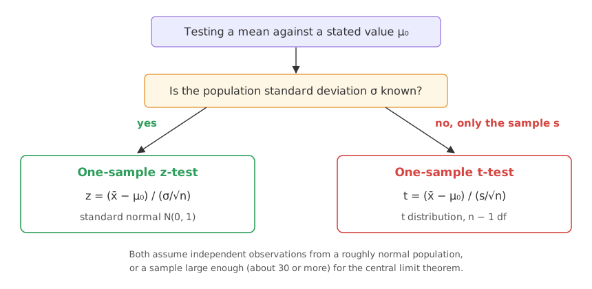
In real data σ is almost never known. The t-test replaces it with the sample's own standard deviation and pays for that estimate with slightly wider critical values.
Choosing a t-test when σ is unknown
The video's rule: whenever the population standard deviation is given, use the One-sample z-test; when it is unknown, use the t-test. Sample size does not decide it. With a large n the t distribution is close to the normal, so the two tests then give nearly the same answer.
Solving the IQ problem with a sample standard deviation
The same question as the z-test: the population's average IQ is 100, and 30 participants who took the medication have a mean IQ of 140. This time only the sample standard deviation is known, s = 20. Did the medication affect intelligence?
- ① Hypotheses: H₀: μ = 100, H₁: μ ≠ 100.
- ② Degrees of freedom: df = n − 1 = 30 − 1 = 29. One degree of freedom is used up because s is measured around the sample's own mean, as in the Sample variance and why n − 1.
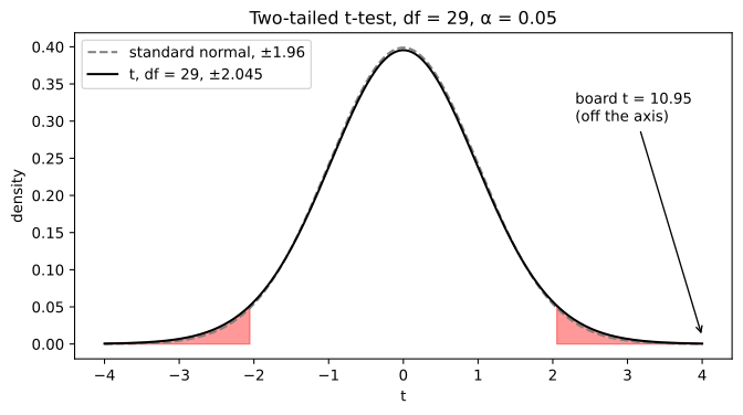
- ③ Decision rule: α = 0.05 and the question allows either direction, so the test is two-tailed with 2.5% in each tail. The t table at df 29 gives ±2.045: reject H₀ if t < −2.045 or t > 2.045.
- ④ Test statistic: t = (x̄ − μ₀)/(s/√n) with x̄ = 140, μ₀ = 100, s = 20, n = 30.
10.95 > 2.045, so we reject H₀: the data are strong evidence that the mean IQ after the medication is not 100, and the positive t says it went up. As the video puts it, rejecting H₀ means the p-value is at most the significance level: t lands in a rejection tail exactly when p ≤ α. Here p is about 8.0 × 10⁻¹²: if the true mean were 100, a sample of 30 with a mean at least 40 points from 100 would almost never be drawn.
Comparing the t distribution with the normal
The t critical value 2.045 is wider than the z value 1.96 for the same α. Estimating σ by s adds uncertainty, so the t distribution has heavier tails than the normal and more of its area lies far out. The fewer the degrees of freedom, the heavier the tails; as df grows, t approaches the standard normal.
import numpy as np
import matplotlib.pyplot as plt
from scipy import stats

x = np.linspace(-4, 4, 400)
crit = stats.t.ppf(0.975, 29)
plt.figure(figsize=(8, 4))
plt.plot(x, stats.norm.pdf(x), "--", color="grey", label="standard normal, ±1.96")
plt.plot(x, stats.t.pdf(x, 29), color="black", label=f"t, df = 29, ±{crit:.3f}")
for tail in (x <= -crit, x >= crit):
    plt.fill_between(x[tail], stats.t.pdf(x[tail], 29), color="red", alpha=0.4)
plt.annotate("board t = 10.95\n(off the axis)", xy=(4, 0.01), xytext=(2.3, 0.3),
             arrowprops=dict(arrowstyle="->"))
plt.title("Two-tailed t-test, df = 29, α = 0.05")
plt.xlabel("t")
plt.ylabel("density")
plt.legend(loc="upper left")
plt.show()
for df in (5, 10, 29, 100, 1000):
    print(f"df {df:4}: critical t = {stats.t.ppf(0.975, df):.3f}")
print(f"normal : critical z = {stats.norm.ppf(0.975):.3f}")df 5: critical t = 2.571 df 10: critical t = 2.228 df 29: critical t = 2.045 df 100: critical t = 1.984 df 1000: critical t = 1.962 normal : critical z = 1.960
The printed critical values shrink from 2.571 at df 5 to 1.962 at df 1000, next to the normal's 1.960. The t table the video reads from shows the same numbers.
Running the one-sample t-test in Python
Computing t from summary numbers
import numpy as np
from scipy import stats

xbar, mu0, s, n = 140, 100, 20, 30     # the board's numbers
t = (xbar - mu0) / (s / np.sqrt(n))
df = n - 1
p_value = 2 * stats.t.sf(abs(t), df)   # two-tailed
Testing raw data with ttest_1samp
The video's notebook has the ages of 32 students and tests whether their mean is 30. It draws a sample of 10 ages. The draw here sets a seed so the run repeats, and takes each student at most once.
ages = [10, 20, 35, 50, 28, 40, 55, 18, 16, 55, 30, 25, 43, 18, 30, 28,
        14, 24, 16, 17, 32, 35, 26, 27, 65, 18, 43, 23, 21, 20, 19, 70]
rng = np.random.default_rng(42)
age_sample = rng.choice(ages, size=10, replace=False)  # 10 different students
result = stats.ttest_1samp(age_sample, popmean=30) # H0: mean age = 30print(f"board: t = {t:.4f}, df = {df}, critical ±{stats.t.ppf(0.975, df):.3f}, p = {p_value:.2g}")
print("all 32 ages, mean:", np.mean(ages))
print("sample:", age_sample, " mean:", age_sample.mean())
print(f"ttest_1samp: t = {result.statistic:.3f}, p = {result.pvalue:.3f}, df = {result.df}")board: t = 10.9545, df = 29, critical ±2.045, p = 8e-12 all 32 ages, mean: 30.34375 sample: [21 16 35 14 25 43 32 50 55 65] mean: 35.6 ttest_1samp: t = 1.024, p = 0.333, df = 9
Testing a class against the school mean
The notebook's second example makes synthetic ages: 18 plus a Poisson count, so the school's mean is about 18 + 35 = 53 and class A's about 18 + 30 = 48. It tests whether class A's mean equals the school's.
import numpy as np
from scipy import stats

np.random.seed(6)
school_ages = stats.poisson.rvs(loc=18, mu=35, size=1500)
classA_ages = stats.poisson.rvs(loc=18, mu=30, size=60)
_, p_value = stats.ttest_1samp(a=classA_ages, popmean=school_ages.mean())
print("class A mean:", classA_ages.mean(), " school mean:", round(school_ages.mean(), 4))
print("p-value:", p_value)
print("reject H0" if p_value <= 0.05 else "fail to reject H0")class A mean: 46.9 school mean: 53.3033 p-value: 1.1390270710161901e-13 reject H0
What the t-test runs printed
- The board's numbers give t = 10.9545 with df 29. The critical value is ±2.045 and p = 8e-12, so H₀ is rejected.
- The 10-age sample has mean 35.6 and p = 0.333. If the mean age of all students were 30, a sample of 10 this far from 30 would happen in about a third of samples. We fail to reject H₀. The full list's mean is 30.34, so that is the right call; a different seed gives a different sample and p.
- Class A's mean 46.9 against the school's 53.3 gives p = 1.14 × 10⁻¹³. We reject H₀: class A's mean age differs from the school's.
Testing one direction: the battery problem
A one-tailed version from the notes that go with the video. A company says its bike batteries last 2 or more years on average. An engineer believes it is less. With 10 batteries the mean life is 1.8 years and the sample standard deviation 0.15. At a 99% confidence level, is there enough evidence to reject the claim?
- Hypotheses: H₀: μ ≥ 2, H₁: μ < 2. Only a low mean counts against H₀, so the whole α sits in the left tail.
- Decision rule: α = 1 − 0.99 = 0.01, df = 9, critical value t = −2.821.
- Statistic: t = (1.8 − 2)/(0.15/√10) = −4.216, below −2.821, so reject H₀.
import numpy as np
from scipy import stats

xbar, mu0, s, n, alpha = 1.8, 2, 0.15, 10, 0.01
t = (xbar - mu0) / (s / np.sqrt(n))
t_crit = stats.t.ppf(alpha, n - 1)          # left tail only
p_value = stats.t.cdf(t, n - 1)             # area to the left of t
print(f"t = {t:.3f}, critical = {t_crit:.3f}, one-sided p = {p_value:.5f}")
print("reject H0" if p_value <= alpha else "fail to reject H0")t = -4.216, critical = -2.821, one-sided p = 0.00113 reject H0
With the raw lifetimes, the same test is stats.ttest_1samp(lifetimes, 2, alternative="less"). One-tailed rules are covered in Significance level, one-tailed and two-tailed tests.
T distribution vs normal distribution
| t distribution | Standard normal | |
|---|---|---|
| Parameter | Degrees of freedom, n − 1 for a one-sample test | None |
| Tails | Heavier; heavier still for small df | Lighter |
| 95% two-tailed critical value | 2.571 (df 5), 2.045 (df 29), 1.984 (df 100) | 1.960 |
| Used by | t-tests, where s estimates σ | z-tests, where σ is known |
Where you use a one-sample t-test
- Checking a claimed average: battery life, delivery time or package weight against what the label promises.
- The Standard Chartered interview question from the video: a bank wants to open an ATM in an area. Frame it as a test on the mean daily withdrawal, H₀: μ ≤ the break-even amount against H₁: μ > it, with a one-tailed t-test on a sample of days.
- Comparing a group with a known benchmark: one class's ages or scores against the school's average.
ttest_1samp's second argument, popmean, is the hypothesized mean μ₀ (30 in the ages example), not a sample size. The test also assumes independent observations from a roughly normal population; with 10 values from a skewed population the p-value can be off, and a rank-based test from Choosing a statistical test is safer.Related
- Previous: One-sample z-test
- Next: Two-sample and paired t-tests
- See also: Confidence intervals
- Reference: scipy.stats.ttest_1samp
- Change the board's s to 80. Is t = 2.74 still beyond 2.045?
- Change the seed in
default_rng(42)to 7 and run again. Does the decision for the 10 ages change? - In the battery example set
alpha = 0.001. Is t = −4.216 still below the new critical value?
Little by little, you're building something great.