
Outlier detection with IQR and z-score
Outlier detection is the process of flagging values that lie far from the rest of the data, here with the IQR fences and with the z-score.
Last updated: 07 Oct, 2026 · SciPy 1.18
Quartiles and the interquartile range and Five-number summary and box plot flagged 27 among 19 values by hand. The same idea runs in Python on a larger dataset here, next to a second method based on the standard deviation, and the two are compared.
Looking at the outlier dataset
The video's dataset has 34 values. Most of them lie between 10 and 19, and three, 102, 107 and 108, are far away. A histogram with ten bins puts 31 values in the first bin and 3 in the last, with nothing in between.
Flagging values beyond three standard deviations
A z-score measures how many standard deviations a value lies from the mean: z = (x − μ)/σ. For data that follows a normal distribution, 99.7% of the values lie within three standard deviations of the mean (Empirical rule (68-95-99.7)), so a value with |z| greater than 3 is unusual and can be treated as an outlier. The z-score has a lesson of its own, Z-score and the standard normal distribution.
The code computes the mean and the standard deviation of the data, works out each value's z-score, and keeps the values whose absolute z-score is above the threshold 3. np.abs takes the absolute value, so a value far below the mean counts the same as one far above it.
The detect_outliers function
def detect_outliers(data):
    outliers = []
    threshold = 3        # 3 standard deviations
    mean = np.mean(data)
    std = np.std(data)
    for i in data:
        z_score = (i - mean) / std
        if np.abs(z_score) > threshold:
            outliers.append(i)
    return outliers
The rule has two weak points on data like this. First, it assumes the data is roughly normal: even clean normal data puts 0.27% of its values beyond three standard deviations. Second, the outliers inflate the very standard deviation used to judge them. The three large values raise it from 2.11 to 26.37, so 102 only reaches z = 3.06, and with a few more outliers the rule could miss all of them. This effect is called masking. With the standard deviation divided by n, as np.std computes it, no z-score in a sample of n values can exceed √(n − 1), which is 5.74 for n = 34.
Flagging values outside the IQR fences
The IQR method follows five steps, the same as in the quartiles lesson:
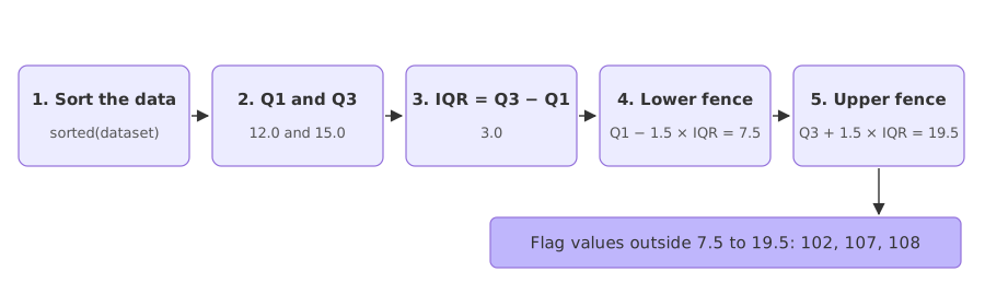
np.percentile(dataset, [25, 75]) returns Q1 = 12.0 and Q3 = 15.0, so the IQR is 3.0 and the fences are 7.5 and 19.5. Any value outside that range is flagged: 102, 107 and 108, the same three as the z-score rule. The fences do not assume a normal distribution, and the outliers barely move them, because quartiles depend on the middle of the data. Sorting is needed for a hand calculation; np.percentile sorts internally. On this data every quantile method gives Q1 = 12 and Q3 = 15, because the values around both quartiles are tied.
The last step is a condition that keeps the values inside the fences: [x for x in dataset if lower_fence <= x <= higher_fence]. Whether to drop a flagged value is a decision, not a rule: a sensor glitch or a typing error should go, a real but rare value should stay.
Drawing the box plot with seaborn
sns.boxplot applies the same 1.5 × IQR rule and draws the three flagged values as separate points. The video passes the list as the first argument, which seaborn 0.13 reads as data and draws as a vertical box; the code here passes x=dataset for the horizontal box the video shows.
Using the modified z-score
A z-score built from the median and the median absolute deviation (MAD, from Range, MAD and coefficient of variation) does not suffer from masking, because neither the median nor the MAD moves much when outliers are added. The modified z-score of Iglewicz and Hoaglin scales the distance from the median by 0.6745/MAD and flags values above 3.5.
Running the z-score rule on the dataset
import numpy as np
import matplotlib.pyplot as plt

dataset = [11, 10, 12, 14, 12, 15, 14, 13, 15, 102, 12, 14, 17, 19, 107,
           10, 13, 12, 14, 12, 108, 12, 11, 14, 13, 15, 10, 15, 12, 10, 14, 13, 15, 10]

counts, edges, bars = plt.hist(dataset)
plt.title("The outlier dataset: 31 values near 10 to 19, 3 far away")
plt.xlabel("value")
plt.ylabel("count")
plt.show()
print("bin counts:", counts)

def detect_outliers(data):
    outliers = []
    threshold = 3        # 3 standard deviations
    mean = np.mean(data)
    std = np.std(data)
    for i in data:
        z_score = (i - mean) / std
        if np.abs(z_score) > threshold:
            outliers.append(i)
    return outliers

print("z-score outliers:", detect_outliers(dataset))
mean, std = np.mean(dataset), np.std(dataset)
print("mean:", round(mean, 2), " std:", round(std, 2))
print("z of 102, 107, 108:", [float(round((v - mean) / std, 2)) for v in (102, 107, 108)])
rest = [v for v in dataset if v < 100]
print("std of the other 31 values:", round(np.std(rest), 2))
print("largest |z| possible with n = 34:", round(np.sqrt(len(dataset) - 1), 2))bin counts: [31. 0. 0. 0. 0. 0. 0. 0. 0. 3.] z-score outliers: [102, 107, 108] mean: 21.18 std: 26.37 z of 102, 107, 108: [3.06, 3.25, 3.29] std of the other 31 values: 2.11 largest |z| possible with n = 34: 5.74
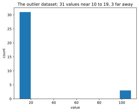
What the z-score run shows
- Bin counts 31 and 3, with eight empty bins between them.
- The z-score rule flags [102, 107, 108], the three values the histogram isolates.
- The mean is 21.18 and the standard deviation 26.37, both pulled up by the outliers; the other 31 values have a standard deviation of 2.11.
- The z-scores are 3.06, 3.25 and 3.29, barely above the threshold of 3: masking at work.
- The largest possible |z| in 34 values is 5.74, so a threshold of 3 leaves little room.
Running the IQR method on the dataset
import numpy as np
import seaborn as sns
import matplotlib.pyplot as plt

dataset = sorted(dataset)
q1, q3 = np.percentile(dataset, [25, 75])
print(q1, q3)
iqr = q3 - q1
print(iqr)
## Find the lower fence and higher fence
lower_fence = q1 - (1.5 * iqr)
higher_fence = q3 + (1.5 * iqr)
print(lower_fence, higher_fence)

flagged = [x for x in dataset if x < lower_fence or x > higher_fence]
kept = [x for x in dataset if lower_fence <= x <= higher_fence]
print("flagged:", flagged, " kept:", len(kept), "values, mean", round(np.mean(kept), 2), "std", round(np.std(kept), 2))

sns.boxplot(x=dataset)
plt.title("Box plot of the outlier dataset")
plt.show()12.0 15.0 3.0 7.5 19.5 flagged: [102, 107, 108] kept: 31 values, mean 13.0 std 2.11
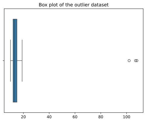
What the IQR run shows
- Q1 = 12.0 and Q3 = 15.0, so the IQR is 3.0.
- The fences are 7.5 and 19.5, the video's numbers.
- Three values are flagged, 102, 107 and 108, and the 31 kept values have a mean of 13.0 and a standard deviation of 2.11.
- The box plot draws the whiskers at 10 and 19, the extremes inside the fences, and the three flagged values as points.
Running the modified z-score on the dataset
import numpy as np
from scipy import stats

median = np.median(dataset)
mad = stats.median_abs_deviation(dataset)
modified_z = 0.6745 * (np.array(dataset) - median) / mad
print("median:", median, " MAD:", mad)
print("flagged (|modified z| > 3.5):", [v for v, m in zip(dataset, modified_z) if abs(m) > 3.5])
print("modified z of 17 and 19:", round(0.6745 * (17 - median) / mad, 2), round(0.6745 * (19 - median) / mad, 2))median: 13.0 MAD: 1.5 flagged (|modified z| > 3.5): [102, 107, 108] modified z of 17 and 19: 1.8 2.7
What the modified z-score shows
- The median is 13.0 and the MAD 1.5, both unaffected by the three large values.
- It flags [102, 107, 108], the same three as the other two methods, with plenty of margin.
- 17 and 19 score 1.8 and 2.7, inside the 3.5 cut-off, as their place in the box plot's whiskers suggests.
IQR vs z-score
| IQR fences | z-score (|z| > 3) | Modified z-score (|M| > 3.5) | |
|---|---|---|---|
| Centre and spread | quartiles | mean and standard deviation | median and MAD |
| Assumes normal data | no | yes | no |
| Masking by outliers | little | strong | little |
| This dataset | 102, 107, 108 | 102, 107, 108 (z = 3.06 to 3.29) | 102, 107, 108 |
| Skewed data | flags many points in the long tail | flags many points in the long tail | flags many points in the long tail |
Where you use outlier detection
- Cleaning sensor and log data, where a glitch writes an impossible value such as a 15-second page load among 3-second ones.
- Before fitting a regression line, because one outlier can tilt it (Simple linear regression).
- Fraud and fault detection, where the outliers are the cases you are looking for and are kept, not removed.
Related
- Previous: Five-number summary and box plot
- Next: Normal (Gaussian) distribution
- See also: Z-score and the standard normal distribution
- Add 120 and 130 to the dataset and run
detect_outliersagain: watch the z-scores of 102, 107 and 108 shrink. - Change
threshold = 3to2and see which values the z-score rule flags. - Change the IQR multiplier from 1.5 to 3 and check whether the three values are still outside the fences.
This is what real progress feels like.