
Hypothesis testing
Hypothesis testing is a method of inferential statistics that uses sample data to decide whether there is enough evidence to reject a null hypothesis H₀ in favour of an alternative hypothesis H₁.
Last updated: 07 Oct, 2026 · SciPy 1.18
The Confidence intervals lesson estimated a mean. Often the question is a yes-or-no one instead: is this coin fair, has the average weight changed, does the new page sell more? A hypothesis test answers it with a rule fixed before the data are seen.
Testing whether a coin is fair
The video's opening problem: you have a coin and want to test whether it is fair by tossing it 100 times. A fair coin has P(H) = 0.5 and P(T) = 0.5. A trick coin like the one in the film Sholay, with heads on both sides, has P(H) = 1, and nobody would call it fair.
With a fair coin, 100 tosses give 50 heads on average. Fifty heads is exactly what a fair coin is expected to produce, so it gives no evidence against fairness. It does not prove fairness either: a coin with P(H) = 0.52 produces 50 heads quite often too. A test can only ask whether the data are surprising enough, if the coin were fair, to doubt it.
Writing the null and alternative hypotheses
- Null hypothesis H₀: the no-effect, status-quo claim, written as an equality. Here H₀: the coin is fair, P(H) = 0.5.
- Alternative hypothesis H₁: what we look for evidence of, the opposite of H₀. Here H₁: the coin is not fair, P(H) ≠ 0.5.
The court analogy fits: a person is presumed innocent (H₀) and cannot be convicted unless the evidence proves guilt beyond reasonable doubt. A not-guilty verdict does not prove innocence; it says the evidence was not strong enough. In the same way a test ends with one of two decisions: reject H₀, or fail to reject H₀.
The steps of a hypothesis test
- State H₀ and H₁ from the question.
- Choose the significance level α, the risk of rejecting a true H₀ you accept, usually 0.05. It is fixed before the data are seen.
- Set the decision boundary: the critical values that cut off a total probability α under H₀ (the rejection region).
- Compute the test statistic from the sample: z, t, χ², or a count such as the number of heads.
- Decide: reject H₀ if the statistic falls in the rejection region, otherwise fail to reject H₀. State the conclusion in the words of the question.
Note the difference between the experiment and the test. The experiment is the data collection (100 tosses). The test is the procedure applied to its result (a z test, a t test, an exact binomial test).
Running the steps on the Bangalore weights
The video's worked problem: the average weight of all residents of Bangalore is 168 pounds, with a standard deviation of 3.9. A sample of 36 individuals has a mean of 169.5 pounds. At the 95% level (α = 0.05), does the sample give evidence that the mean weight is different?
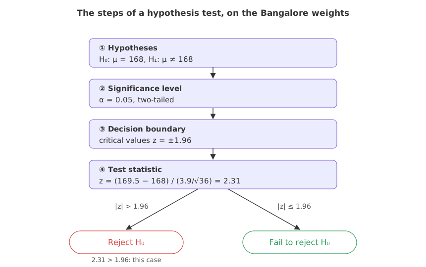
- Hypotheses: H₀: μ = 168, H₁: μ ≠ 168. "Different" points both ways, so the test is two-tailed.
- Significance level: α = 0.05, split as 0.025 in each tail.
- Decision boundary: the z-table gives 1.96 for a left area of 1 − 0.025 = 0.975, so the critical values are ±1.96.
- Test statistic: with σ known, z = (x̄ − μ₀)/(σ/√n) = (169.5 − 168)/(3.9/√36) = 1.5/0.65 = 2.31.
- Decision: 2.31 > 1.96, so z falls in the rejection region and H₀ is rejected.
Conclusion in the question's words: at the 5% level, the sample gives evidence that the mean weight of Bangalore residents differs from 168 pounds. The Z-score and the standard normal distribution lesson introduced the z scale; the One-sample z-test lesson covers this test in full.
import math
from scipy.stats import norm

mu0, sigma, n, xbar = 168, 3.9, 36, 169.5   # H0: mu = 168, sigma known
alpha = 0.05

se = sigma / math.sqrt(n)
z = (xbar - mu0) / se                        # the test statistic
crit = norm.ppf(1 - alpha / 2)               # two-tailed critical value
print("SE =", round(se, 3), "  z =", round(z, 4), "  critical values = ±" + str(round(crit, 3)))
print("reject H0" if abs(z) > crit else "fail to reject H0")SE = 0.65 z = 2.3077 critical values = ±1.96 reject H0
Testing the fair coin with the exact binomial distribution
For the coin, the test statistic is the number of heads X. If H₀ is true, X follows a Binomial distribution with n = 100 and p = 0.5: mean np = 50 and standard deviation √(np(1 − p)) = √25 = 5. The rejection region at α = 0.05 collects the most extreme counts on both sides, at most 0.025 in each tail.
The number of heads under H₀
from scipy.stats import binom
heads = binom(100, 0.5)            # X = heads in 100 tosses of a fair coin
print(heads.mean(), heads.std())   # 50.0 5.0
Finding the rejection region
import numpy as np
k = np.arange(101)
lo = k[heads.cdf(k) <= 0.025].max()      # largest k with P(X <= k) <= 0.025
hi = k[heads.sf(k - 1) <= 0.025].min()   # smallest k with P(X >= k) <= 0.025
Then each observed count is checked against the region:
print("mean", heads.mean(), "  SD", heads.std())
print("reject H0 when heads <=", lo, "or heads >=", hi)
print("chance of landing there with a fair coin:", round(heads.cdf(lo) + heads.sf(hi - 1), 4))
for x in (10, 30, 50, 60, 95):
print(f"{x:2} heads:", "reject H0" if (x <= lo or x >= hi) else "fail to reject H0")mean 50.0 SD 5.0 reject H0 when heads <= 39 or heads >= 61 chance of landing there with a fair coin: 0.0352 10 heads: reject H0 30 heads: reject H0 50 heads: fail to reject H0 60 heads: fail to reject H0 95 heads: reject H0
import numpy as np
import matplotlib.pyplot as plt
from scipy.stats import binom

k = np.arange(101)
pmf = binom.pmf(k, 100, 0.5)
reject = (k <= 39) | (k >= 61)               # the region found above
plt.figure(figsize=(8, 4))
plt.bar(k[~reject], pmf[~reject], color="tab:blue", label="fail to reject H0: 40 to 60 heads")
plt.bar(k[reject], pmf[reject], color="red", label="reject H0: 39 or fewer, 61 or more")
for x in (10, 30, 50, 60, 95):
    plt.axvline(x, color="grey", linestyle=":")
plt.title("Heads in 100 tosses of a fair coin: Binomial(100, 0.5)")
plt.xlabel("number of heads")
plt.ylabel("probability")
plt.legend(loc="upper left", fontsize=9)
plt.show()
print("P(40 to 60 heads) =", round(pmf[~reject].sum(), 4))P(40 to 60 heads) = 0.9648
What the coin test decided
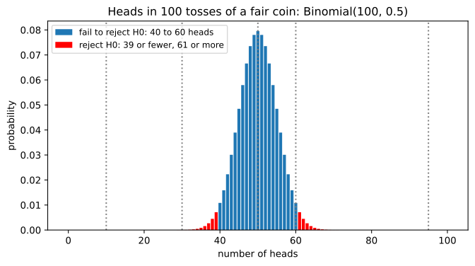
- The rejection region is 39 or fewer heads, or 61 or more. A fair coin lands there with probability 0.0352, a little under α = 0.05, because a count cannot be split.
- 10, 30 and 95 heads reject H₀: each is far outside the range a fair coin produces. Thirty heads is 4 standard deviations below 50.
- 50 heads fails to reject H₀: no evidence the coin is unfair, which is not proof that it is fair.
- 60 heads also fails to reject H₀, by the smallest margin: 61 would have rejected it. A borderline result is weak evidence, not a clean bill of health.
- About 96% of a fair coin's results fall between 40 and 60 heads (0.9648).
Rejecting H₀ vs failing to reject H₀
| Reject H₀ | Fail to reject H₀ | |
|---|---|---|
| When | The statistic is in the rejection region | The statistic is outside it |
| What it means | The data would be surprising if H₀ were true | The data are compatible with H₀ |
| What it does not mean | H₁ is certainly true | H₀ is true |
| Fair coin, α = 0.05 | 30 heads | 50 or 60 heads |
| Possible error | Type I: rejecting a true H₀ | Type II: failing to reject a false H₀ |
Where you use hypothesis testing
- Quality control: a machine should fill 80 ml bottles; a sample mean of 78 ml over 40 bottles tests whether it is off.
- A/B testing: H₀ says the new checkout page converts at the same rate as the old one.
- Medical trials: H₀ says the drug works no better than a placebo; the trial looks for evidence against it.
Related
- Previous: Confidence intervals
- Next: P-value
- Reference: scipy.stats.binomtest
- Change the Bangalore sample mean to
xbar = 168.9. What is z now, and what is the decision? - Use α = 0.01 for the coin: replace both
0.025with0.005. What is the new region, and does 60 heads change? - Test 1,000 tosses:
binom(1000, 0.5)andnp.arange(1001). Is 530 heads in the rejection region?
Little by little, you're building something great.