
Z-table and normal probabilities
A z-table is a table of standard normal probabilities: for each z-score it gives Φ(z), the area under the curve to the left of z, which is the share of values below it.
Last updated: 07 Oct, 2026 · SciPy 1.18
Z-score and the standard normal distribution turned every normal distribution into the standard normal. One table of the standard normal therefore answers "what share lies above, below or between" for any normal distribution.
Finding the share of scores above 4.25
The video's interview question: scores follow a normal distribution with mean 4 and standard deviation 1. What percentage of the scores fall above 4.25?
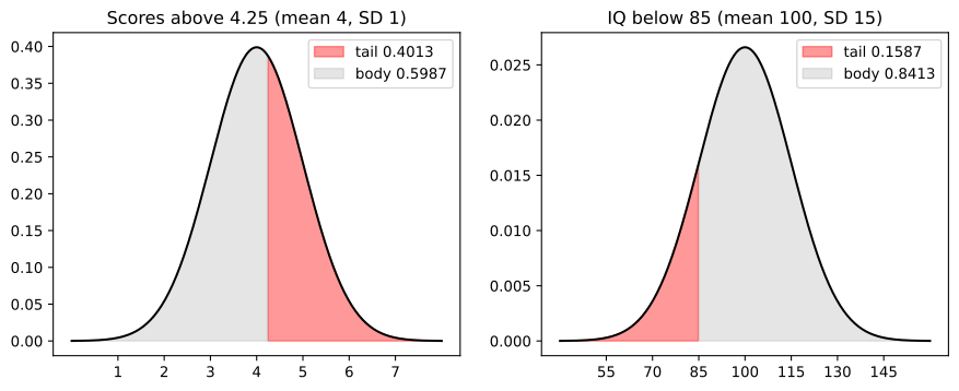
First the z-score: z = (4.25 − 4)/1 = 0.25, so 4.25 lies 0.25 standard deviations above the mean. The whole area under the curve is 1. The region the question asks about, to the right of 4.25, is the tail; the rest, to the left of 4.25, is the body. The z-score is what lets one table give the area of either part.
Reading the left z-table
A left (cumulative) z-table lists Φ(z) = P(Z ≤ z). The row is z to one decimal and the column is its second decimal, so z = 0.25 is row 0.2, column .05: 0.5987. That is the body, the share of scores below 4.25. The tail is the rest of the total area of 1:
So 40.13% of the scores fall above 4.25.
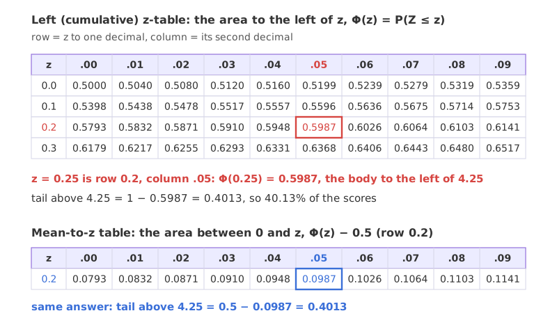
Some tables give a different area. A mean-to-z table lists the area between 0 and z, which is Φ(z) − 0.5. Its row 0.2, column .05 holds 0.0987, so the tail is 0.5 − 0.0987 = 0.4013, the same answer by a second route. Read a table's heading before you use it.
Finding the share with an IQ below 85
The video's second question: in India the average IQ is 100, with a standard deviation of 15. What percentage of the population would you expect to have an IQ lower than 85?
z = (85 − 100)/15 = −15/15 = −1, one standard deviation below the mean. The region below 85 is the left tail. A table of positive z gives Φ(1) = 0.84134, and by symmetry the area left of −1 equals the area right of +1:
About 15.87% of the population has an IQ below 85, and the body, 84.13%, lies above it. For a continuous variable P(IQ < 85) and P(IQ ≤ 85) are the same number.
Finding the share between two values
The video leaves one more question as an exercise: what share has an IQ between 90 and 120? Take the area left of 120 and subtract the area left of 90:
About 65.63% of people have an IQ between 90 and 120.
Comparing two series with z-scores
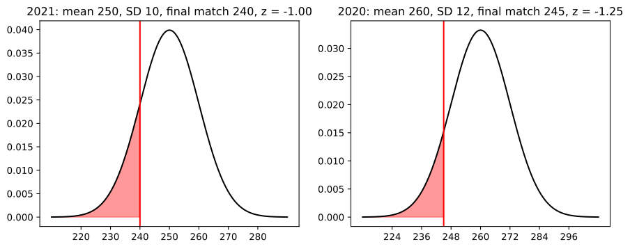
Earlier in the video, z-scores compare India's showing in two ODI series. In the 2021 series the average score was 250 with a standard deviation of 10, and the score in the final match was 240. In the 2020 series the average was 260 with a standard deviation of 12, and the final-match score was 245. In which year was the final-match score better, compared with its own series?
Both scores are below their series average, but the 2021 score is less far below: −1 is higher than −1.25. As percentiles, Φ(−1) = 15.87% of 2021 scores would be lower than 240, against Φ(−1.25) = 10.56% of 2020 scores lower than 245. Relative to its own series, the 2021 final was the better performance. The comparison assumes each series' scores are roughly normal.
Computing normal probabilities with scipy
The area to the left with norm.cdf
norm.cdf is the left z-table. With loc and scale it works on the original scale, so the z-score step is done for you.
from scipy.stats import norm

norm.cdf(0.25)                          # area left of z = 0.25, the body
norm.cdf(85, loc=100, scale=15)         # area left of IQ 85, no z-score needed
The area to the right with norm.sf
sf is the survival function, 1 − cdf. It is also more accurate than 1 − cdf far out in a tail.
norm.sf(0.25) # area right of z = 0.25, 1 - cdfA value from an area with norm.ppf
ppf, the percent point function, runs the table backwards: give it an area and it returns the value with that area to its left.
norm.ppf(0.95, loc=100, scale=15) # the IQ that 95% of people fall belowz = (4.25 - 4) / 1
print("4.25: z =", z, " body", round(norm.cdf(z), 4), " tail", round(norm.sf(z), 4))
z = (85 - 100) / 15
print("85: z =", z, " Phi(-1) =", round(norm.cdf(z), 5), " 1 - Phi(1) =", round(1 - norm.cdf(1), 5))
lo, hi = norm.cdf(90, loc=100, scale=15), norm.cdf(120, loc=100, scale=15)
print("90 to 120:", round(hi, 4), "-", round(lo, 4), "=", round(hi - lo, 4))
print("top 5% IQ cut-off:", round(norm.ppf(0.95, loc=100, scale=15), 1))
print("z with 97.5% below:", round(norm.ppf(0.975), 2))4.25: z = 0.25 body 0.5987 tail 0.4013 85: z = -1.0 Phi(-1) = 0.15866 1 - Phi(1) = 0.15866 90 to 120: 0.9088 - 0.2525 = 0.6563 top 5% IQ cut-off: 124.7 z with 97.5% below: 1.96
Building z-table rows from norm.cdf
import numpy as np

columns = np.arange(10) / 100                       # .00 to .09
for row in [0.0, 0.1, 0.2, 0.3, 1.0]:
print(f"{row:.1f}", " ".join(f"{norm.cdf(row + c):.4f}" for c in columns))0.0 0.5000 0.5040 0.5080 0.5120 0.5160 0.5199 0.5239 0.5279 0.5319 0.5359 0.1 0.5398 0.5438 0.5478 0.5517 0.5557 0.5596 0.5636 0.5675 0.5714 0.5753 0.2 0.5793 0.5832 0.5871 0.5910 0.5948 0.5987 0.6026 0.6064 0.6103 0.6141 0.3 0.6179 0.6217 0.6255 0.6293 0.6331 0.6368 0.6406 0.6443 0.6480 0.6517 1.0 0.8413 0.8438 0.8461 0.8485 0.8508 0.8531 0.8554 0.8577 0.8599 0.8621
These are the rows of a printed left z-table, computed rather than copied: row 0.2 holds 0.5987 under .05, and row 1.0 starts with 0.8413, the Φ(1) used for the IQ question.
Shading the tail and the body
import numpy as np
import matplotlib.pyplot as plt

fig, axes = plt.subplots(1, 2, figsize=(11, 4))
cases = [(axes[0], 4, 1, 4.25, "right", "Scores above 4.25 (mean 4, SD 1)"),
         (axes[1], 100, 15, 85, "left", "IQ below 85 (mean 100, SD 15)")]
for ax, mu, sd, cut, side, title in cases:
    x = np.linspace(mu - 4 * sd, mu + 4 * sd, 400)
    tail = x >= cut if side == "right" else x <= cut
    area = norm.sf(cut, mu, sd) if side == "right" else norm.cdf(cut, mu, sd)
    ax.plot(x, norm.pdf(x, mu, sd), color="black")
    ax.fill_between(x[tail], norm.pdf(x[tail], mu, sd), color="red", alpha=0.4, label=f"tail {area:.4f}")
    ax.fill_between(x[~tail], norm.pdf(x[~tail], mu, sd), color="grey", alpha=0.2, label=f"body {1 - area:.4f}")
    ax.set_xticks([mu + k * sd for k in range(-3, 4)])
    ax.set_title(title)
    ax.legend()
    print(f"{title}: tail {area:.4f}, body {1 - area:.4f}")
plt.show()Scores above 4.25 (mean 4, SD 1): tail 0.4013, body 0.5987 IQ below 85 (mean 100, SD 15): tail 0.1587, body 0.8413
Comparing the two cricket series in code
import numpy as np
import matplotlib.pyplot as plt

fig, axes = plt.subplots(1, 2, figsize=(11, 4))
for ax, (year, mu, sd, score) in zip(axes, [(2021, 250, 10, 240), (2020, 260, 12, 245)]):
    z = (score - mu) / sd
    print(f"{year}: z = {z:+.2f}, share of series scores below {score} = {norm.cdf(z):.2%}")
    x = np.linspace(mu - 4 * sd, mu + 4 * sd, 400)
    below = x <= score
    ax.plot(x, norm.pdf(x, mu, sd), color="black")
    ax.fill_between(x[below], norm.pdf(x[below], mu, sd), color="red", alpha=0.4)
    ax.axvline(score, color="red")
    ax.set_xticks([mu + k * sd for k in range(-3, 4)])
    ax.set_title(f"{year}: mean {mu}, SD {sd}, final match {score}, z = {z:.2f}")
plt.show()2021: z = -1.00, share of series scores below 240 = 15.87% 2020: z = -1.25, share of series scores below 245 = 10.56%
What the probabilities show
- 4.25 gives z = 0.25, body 0.5987 and tail 0.4013: 40.13% of the scores fall above 4.25, as in the table.
- 85 gives z = −1.0 and Φ(−1) = 0.15866, equal to 1 − Φ(1): the symmetry step from the IQ question.
- 90 to 120 gives 0.9088 − 0.2525 = 0.6563.
- norm.ppf(0.95) on the IQ scale is 124.7: the top 5% of people have an IQ above about 124.7. On the standard scale, norm.ppf(0.975) = 1.96, the z with 2.5% above it.
- 2021 gives z = −1.00 with 15.87% of scores below it; 2020 gives z = −1.25 with 10.56%, so the 2021 final ranks higher within its series.
norm.cdf vs norm.sf vs norm.ppf
| Function | Gives | Example | Result |
|---|---|---|---|
| norm.cdf(x) | Area left of x, P(X ≤ x) | norm.cdf(0.25) | 0.5987 |
| norm.sf(x) | Area right of x, 1 − cdf | norm.sf(0.25) | 0.4013 |
| norm.ppf(p) | The x with area p to its left (inverse of cdf) | norm.ppf(0.95, 100, 15) | 124.7 |
| norm.cdf(b) − norm.cdf(a) | Area between a and b | IQ 90 to 120 | 0.6563 |
Where you use normal probabilities
- P-values. The area beyond a test statistic is a p-value; P-value reads it off the same curve.
- Critical values. norm.ppf(0.975) = 1.96 sets the edges of a 95% interval in Confidence intervals.
- Percentiles of scores. Exam and IQ results are reported this way: an IQ of 85 sits at about the 16th percentile.
norm.cdf give the area below z; for "above", take 1 − Φ(z) or norm.sf. A quick sketch of the curve with the wanted area shaded catches most mistakes.Related
- Previous: Standardization and normalization
- Next: Normality tests (Q-Q plot and Shapiro-Wilk)
- See also: P-value
- Reference: scipy.stats.norm
- Find the share of scores below 3.5 for mean 4 and SD 1: z = −0.5, and
norm.cdf(-0.5)gives 0.3085. - Solve P(90 < IQ < 120) from the printed table by rounding z to 1.33 and −0.67: Φ(1.33) − Φ(−0.67) = 0.9082 − 0.2514 = 0.6568, close to scipy's 0.6563.
- Change the 2020 standard deviation from 12 to 20 in the cricket example: z becomes −0.75, and the 2020 final now ranks higher than the 2021 one.
This is what real progress feels like.