
Spearman rank correlation
Spearman's rank correlation coefficient is a measure of the strength and direction of a monotonic relationship between two variables: the Pearson correlation computed on the ranks of the values instead of the values themselves.
Last updated: 07 Oct, 2026 · SciPy 1.18
The Pearson correlation coefficient asks how close the points are to a straight line. Many relationships are not straight but still always go one way: more experience, higher salary, but with diminishing steps. Spearman's correlation measures that.
Seeing where Pearson falls short
The video's figure shows points where y rises every time x rises, quickly at first and then by small amounts. Pearson gives 0.88 there, not 1, because the points do not lie on a line. A relationship like this, where y only ever rises (or only ever falls) as x rises, is called monotonic. It need not be linear. Spearman's correlation is 1 for any perfectly rising monotonic relationship and −1 for any perfectly falling one.
import numpy as np
import matplotlib.pyplot as plt
from scipy import stats

x = np.linspace(0, 1, 40)
y = np.exp(6 * x)                            # always rising, but not a straight line
r = stats.pearsonr(x, y).statistic
r_s = stats.spearmanr(x, y).statistic
plt.figure(figsize=(6, 4))
plt.scatter(x, y, s=15)
plt.title(f"A monotonic curve: Pearson r = {r:.2f}, Spearman = {r_s:.2f}")
plt.xlabel("x")
plt.ylabel("y = exp(6x)")
plt.show()
print(f"Pearson {r:.3f}, Spearman {r_s:.3f}")Pearson 0.814, Spearman 1.000
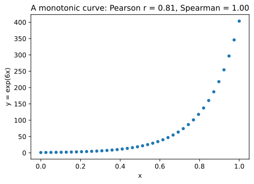
The curve never goes down, so the ranks of x and y agree perfectly and Spearman is 1.00, while Pearson is pulled below 1 by the bend.
Ranking the values
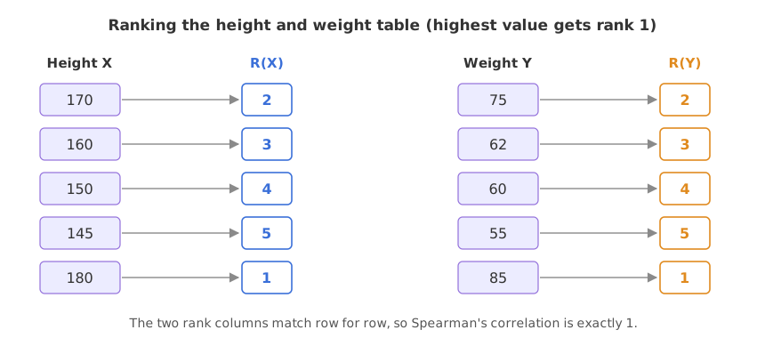
Spearman replaces every value by its rank and then computes Pearson's formula on the ranks: the covariance of the ranks divided by the standard deviations of the ranks. The board's example adds a fifth person to the height and weight table and ranks each column with the highest value as rank 1.
When no values are tied there is a shortcut using d, the difference between a row's two ranks:
Ranking from the highest or from the lowest gives the same r_s, as long as both columns are ranked the same way. In the board's table every d is 0, so r_s = 1 − 0 = 1.
Computing Spearman correlation in Python
Ranks with rankdata
import numpy as np
from scipy import stats

height = np.array([170, 160, 150, 145, 180])
weight = np.array([75, 62, 60, 55, 85])
rank_h = stats.rankdata(-height)        # highest height gets rank 1, as on the board
rank_w = stats.rankdata(-weight)print("R(height):", rank_h, " R(weight):", rank_w)
print("Pearson on the ranks:", round(stats.pearsonr(rank_h, rank_w).statistic, 5))
print("spearmanr:", round(stats.spearmanr(height, weight).statistic, 5))
print("Pearson on the raw values:", round(stats.pearsonr(height, weight).statistic, 5))R(height): [2. 3. 4. 5. 1.] R(weight): [2. 3. 4. 5. 1.] Pearson on the ranks: 1.0 spearmanr: 1.0 Pearson on the raw values: 0.97663
- Both rank columns print as 2, 3, 4, 5, 1, the board's ranks.
- Pearson on the ranks and spearmanr both give 1.0. The order of the heights matches the order of the weights exactly.
- Pearson on the raw values is 0.97663: high, but below 1, because the points are not on one straight line.
The marks example with the shortcut
The notes that go with the video rank a second table, X = 1, 3, 7, 0, 8 and Y = 2, 4, 5, 7, 1, with ranks R_x = 4, 3, 2, 5, 1 and R_y = 4, 3, 2, 1, 5. The last two rows swap places, so d = 0, 0, 0, 4, −4 and Σd² = 32:
import numpy as np
from scipy import stats

X = np.array([1, 3, 7, 0, 8])
Y = np.array([2, 4, 5, 7, 1])
d = stats.rankdata(-X) - stats.rankdata(-Y)       # rank differences
n = len(X)
r_s = 1 - 6 * (d ** 2).sum() / (n * (n ** 2 - 1))
print("ranks X:", stats.rankdata(-X), " ranks Y:", stats.rankdata(-Y))
print("sum of d^2:", (d ** 2).sum(), " shortcut r_s:", round(r_s, 4))
print("spearmanr:", round(stats.spearmanr(X, Y).statistic, 4),
" Pearson:", round(stats.pearsonr(X, Y).statistic, 4))ranks X: [4. 3. 2. 5. 1.] ranks Y: [4. 3. 2. 1. 5.] sum of d^2: 32.0 shortcut r_s: -0.6 spearmanr: -0.6 Pearson: -0.4466
Ties get average ranks
When two values are equal they share the average of the ranks they would take. The shortcut formula is then only approximate, while spearmanr stays exact because it computes Pearson on the average ranks.
from scipy import stats

ratings = [5, 3, 3, 4, 1]                    # two people gave 3
print("average ranks:", stats.rankdata(ratings))average ranks: [5. 2.5 2.5 4. 1. ]
Comparing Spearman and Pearson on outliers and curves
import numpy as np
from scipy import stats

rng = np.random.default_rng(42)
x = np.arange(1, 21)
y = x + rng.normal(0, 2, 20)
y_out = y.copy()
y_out[-1] = -60                              # one wrong entry
u = np.linspace(-2, 2, 21)
for name, a, b in (("clean", x, y), ("one outlier", x, y_out), ("U-shape", u, u ** 2)):
    print(f"{name:12} Pearson {stats.pearsonr(a, b).statistic:6.3f}   "
f"Spearman {stats.spearmanr(a, b).statistic:6.3f}")clean Pearson 0.964 Spearman 0.962 one outlier Pearson -0.032 Spearman 0.678 U-shape Pearson 0.000 Spearman 0.042
On clean, roughly linear data the two agree. One wrong entry drags Pearson far down, while Spearman, which only sees that the point has the lowest rank, moves much less. On a U-shape both are near 0: Spearman captures curves that keep one direction, not every non-linear relationship.
Spearman vs Pearson correlation
| Spearman r_s | Pearson r | |
|---|---|---|
| Measures | monotonic association | linear association |
| Computed on | the ranks | the values |
| Outliers | little effect | can change r a lot |
| Data | numeric or ordinal | numeric |
| Board's height and weight | 1.0 | 0.977 |
| Python | spearmanr, df.corr(method="spearman") | pearsonr, df.corr() |
Where you use Spearman rank correlation
- Ordinal data: ratings, survey answers on a 1 to 5 scale, or rankings from two judges.
- Skewed data with outliers: income, house prices or page-load times, where a few large values dominate Pearson.
- Monotonic but curved relationships: dose and response, experience and salary.
Related
- Previous: Pearson correlation coefficient
- Next: Statistics interview questions
- Reference: scipy.stats.spearmanr
- In the board's table change the 180 cm person's weight to 50 kg. What happens to Spearman and to Pearson?
- Run
stats.kendalltau(height, weight), another rank correlation, on the board's table. - In the curve example replace
np.exp(6 * x)withnp.sin(6 * x). Why does Spearman drop below 1?
Every expert started right here.