
Central limit theorem
The central limit theorem is the result that the mean of a large random sample of independent values from one distribution with finite variance has an approximately normal distribution, whatever the shape of that distribution.
Last updated: 07 Oct, 2026 · SciPy 1.18
The distributions in this part come in many shapes: skewed, flat, discrete, heavy-tailed. Yet the z-tests, t-tests and Confidence intervals later on all use normal or t curves. The central limit theorem (CLT) is the reason: they work with sample means, and sample means are close to normal.
Taking many samples and their means
Start with a population whose distribution may be normal, or not normal, or any other shape. Take a random sample of size n, with n ≥ 30 in the video, and compute its mean x̄₁. Take another sample and compute x̄₂, and so on up to x̄ₘ for m samples. Plot all the sample means, and they form an approximately normal distribution.
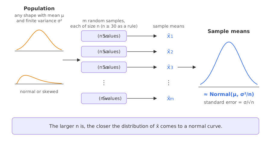
Two numbers play different parts. The sample size n is the number of values in each sample: the larger n is, the closer the means come to a normal curve. The number of samples m only decides how many means you plot: a larger m draws the shape more clearly, but does not change the shape.
Stating the theorem with its conditions
Let X₁, X₂, …, Xₙ be independent random values from the same distribution, with mean μ and a finite variance σ². Then for large n the sample mean has an approximately normal distribution:
- Independent values from one distribution (i.i.d.): a random sample, not values that influence each other.
- A finite variance: the population's spread must exist. Almost every distribution met in practice has one; the Pareto distribution with α ≤ 2 does not.
- A large enough n: n ≥ 30 is a rule of thumb. A symmetric population needs fewer values; a strongly skewed one needs more.
The means are centred on the population mean μ, and their spread, the standard error σ/√n, shrinks as n grows: four times the data halves the standard error.
Watching the theorem work on a skewed population
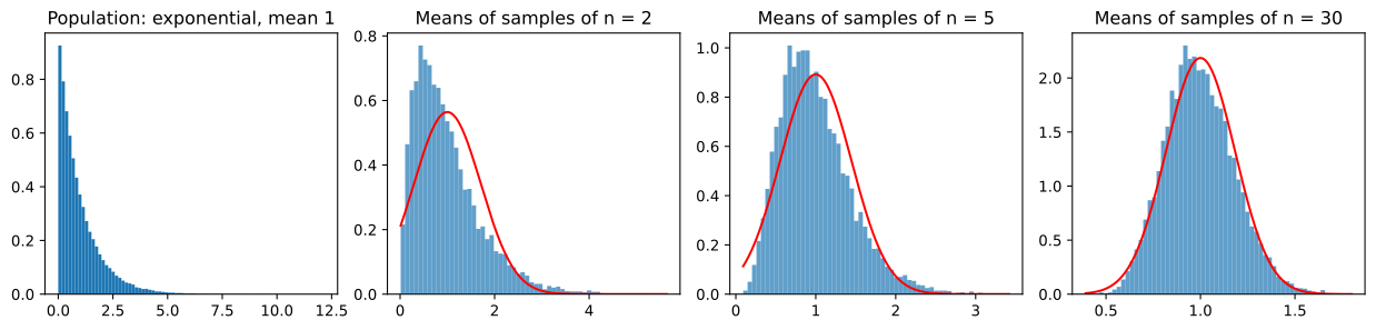
An exponential population with mean 1 is strongly right-skewed (skewness 2) and has σ = 1. The code takes m = 10,000 samples for n = 2, 5 and 30, and compares the spread of their means with σ/√n.
import numpy as np
import matplotlib.pyplot as plt
from scipy import stats

rng = np.random.default_rng(42)
fig, ax = plt.subplots(1, 4, figsize=(13, 3.2))
ax[0].hist(rng.exponential(1, 100_000), bins=80, density=True)
ax[0].set_title("Population: exponential, mean 1")
for a_, n in zip(ax[1:], (2, 5, 30)):
    means = rng.exponential(1, size=(10_000, n)).mean(axis=1)   # 10,000 samples of size n
    print(f"n = {n:>2}: mean of means {means.mean():.3f}  sd {means.std(ddof=1):.3f}  sigma/sqrt(n) {1 / np.sqrt(n):.3f}  skew {stats.skew(means):.2f}")
    a_.hist(means, bins=60, density=True, alpha=0.7)
    t = np.linspace(means.min(), means.max(), 300)
    a_.plot(t, stats.norm.pdf(t, 1, 1 / np.sqrt(n)), color="red")
    a_.set_title(f"Means of samples of n = {n}")
fig.tight_layout()
plt.show()n = 2: mean of means 0.998 sd 0.712 sigma/sqrt(n) 0.707 skew 1.40 n = 5: mean of means 0.996 sd 0.442 sigma/sqrt(n) 0.447 skew 0.89 n = 30: mean of means 0.996 sd 0.183 sigma/sqrt(n) 0.183 skew 0.31
What the sample means show
- The means are centred on μ = 1 for every n: 0.998, 0.996 and 0.996.
- Their spread matches σ/√n: 0.712 vs 0.707 for n = 2, 0.442 vs 0.447 for n = 5, 0.183 vs 0.183 for n = 30.
- The skew fades as n grows: 1.40 for n = 2, 0.89 for n = 5 and 0.31 for n = 30, down from 2 in the population. At n = 30 the histogram sits close to the normal curve; a more skewed population would need a larger n.
Seeing the theorem fail without finite variance
The Power law and Pareto distribution with α = 1.5 has a mean of 3 but an infinite variance, so the second condition fails. The same experiment with n = 30 gives means that stay heavily skewed.
import numpy as np
from scipy import stats

rng = np.random.default_rng(42)
pareto_means = stats.pareto.rvs(b=1.5, size=(10_000, 30), random_state=rng).mean(axis=1)
expo_means = rng.exponential(1, size=(10_000, 30)).mean(axis=1)
print("population mean of Pareto(1.5):", stats.pareto(b=1.5).mean(), "  variance:", stats.pareto(b=1.5).var())
print("Pareto means, n = 30:      median", round(np.median(pareto_means), 3), " skew", round(stats.skew(pareto_means), 1), " largest", round(pareto_means.max(), 1))
print("exponential means, n = 30: median", round(np.median(expo_means), 3), " skew", round(stats.skew(expo_means), 2))population mean of Pareto(1.5): 3.0 variance: inf Pareto means, n = 30: median 2.528 skew 35.6 largest 204.0 exponential means, n = 30: median 0.986 skew 0.4
- The Pareto population has mean 3.0 and variance inf: the condition of a finite variance fails.
- Its sample means are not normal: their skewness is 35.6, one sample of 30 values has a mean of 204.0, and the median of the means, 2.528, sits below the population mean of 3.
- The exponential means at the same n are close to symmetric, with a skewness of 0.4, as in the previous run.
The population vs the distribution of sample means
| Population (the data) | Sample means (x̄) | |
|---|---|---|
| Shape | Any: skewed, flat, discrete | Close to normal for large n |
| Centre | μ | μ |
| Spread | σ | σ/√n, the standard error |
| Changes with n? | No | Narrower and more normal as n grows |
Where you use the central limit theorem
- Confidence intervals and tests for a mean: One-sample z-test and One-sample t-test and the t distribution treat x̄ as normal with standard error σ/√n.
- Proportions: a sample proportion is a mean of 0s and 1s, so it is close to N(p, p(1 − p)/n), the basis of the Z-test for a proportion.
- A/B tests and monitoring: averages of skewed quantities, such as order values or load times, are compared with normal-theory methods.
Related
- Replace the exponential with a uniform population,
rng.uniform(0, 1, size=(10_000, n)), and σ/√n withnp.sqrt(1 / 12) / np.sqrt(n). How small an n already looks normal? - Change n = 30 to n = 120 in the first example. Does the standard error halve to about 0.091?
- Run the Pareto experiment with
b=3, which has a finite variance. Does the skew of the means fall?
Slow is fine. Stopping is the only problem.