
Chi-square test of independence
A chi-square test of independence is a hypothesis test that checks whether two categorical variables are related, by comparing the counts in their contingency table with the counts expected if they were independent.
Last updated: 07 Oct, 2026 · SciPy 1.18
The Chi-square goodness-of-fit test tested one variable against stated shares. The video's notebook asks a question about two variables at once: in a restaurant's tips data, is being a smoker related to the diner's sex?
Building the contingency table
A contingency table (a crosstab) counts every combination of the two variables: rows for one variable, columns for the other. The notebook builds it from seaborn's tips dataset, 244 restaurant bills.
import pandas as pd
import seaborn as sns
from scipy import stats

dataset = sns.load_dataset("tips")
dataset_table = pd.crosstab(dataset["sex"], dataset["smoker"])
print(dataset_table)
The table has Male: 60 smokers and 97 non-smokers, Female: 33 and 54. The hypotheses are H₀: sex and smoking are independent, and H₁: they are related.
Computing expected counts under independence
If the two variables were independent, the share of smokers would be the same for men and women: the overall share, 93 of 244. So the expected count for a cell is its row total times its column total divided by the grand total N. For Male and smoker: 157 × 93 / 244 = 59.84.
| Smoker: Yes | Smoker: No | Row total | |
|---|---|---|---|
| Male, observed (expected) | 60 (59.84) | 97 (97.16) | 157 |
| Female, observed (expected) | 33 (33.16) | 54 (53.84) | 87 |
| Column total | 93 | 151 | 244 |
Every observed count is within 0.16 of its expected count. A 2 × 2 table has (2 − 1)(2 − 1) = 1 degree of freedom: once one cell is fixed, the totals fix the other three.
Running the test by hand
The notebook computes the statistic, the critical value and the p-value itself. Here is the same calculation with the expected counts written out from the formula above.
Observed counts, expected counts and the statistic
observed = dataset_table.values
row_totals = observed.sum(axis=1, keepdims=True)
col_totals = observed.sum(axis=0, keepdims=True)
expected = row_totals * col_totals / observed.sum()   # row total x column total / N
chi_square = ((observed - expected) ** 2 / expected).sum()
ddof = (observed.shape[0] - 1) * (observed.shape[1] - 1)alpha = 0.05
critical_value = stats.chi2.ppf(q=1 - alpha, df=ddof)
p_value = stats.chi2.sf(chi_square, df=ddof)
print("expected:\n", expected.round(2))
print(f"chi-square = {chi_square:.6f}, df = {ddof}, critical = {critical_value:.3f}, p = {p_value:.4f}")
print("reject H0" if p_value <= alpha else "fail to reject H0: no evidence of a relationship")expected: [[59.84 97.16] [33.16 53.84]] chi-square = 0.001935, df = 1, critical = 3.841, p = 0.9649 fail to reject H0: no evidence of a relationship
χ² = 0.001935 is far below the critical 3.841, and p = 0.9649. If sex and smoking were independent, a table at least this far from the expected counts would turn up in about 96% of samples of 244. We fail to reject H₀: the data show no relationship between sex and smoking.
Running chi2_contingency and the Yates correction
scipy.stats.chi2_contingency does the whole test in one call. On a 2 × 2 table it applies Yates' continuity correction by default (correction=True): it moves every observed count 0.5 closer to its expected count before squaring, to make the χ² approximation less eager to reject on small tables. SciPy never moves a count past its expected value, so when |O − E| is under 0.5 the corrected gap is 0.
with_yates = stats.chi2_contingency(dataset_table)                   # correction=True by default
no_yates = stats.chi2_contingency(dataset_table, correction=False)
print("default (Yates):  ", round(with_yates.statistic, 6), round(with_yates.pvalue, 4), with_yates.dof)
print("correction=False: ", round(no_yates.statistic, 6), round(no_yates.pvalue, 4), no_yates.dof)
print("largest |O - E|: ", round(abs(dataset_table.values - with_yates.expected_freq).max(), 3))default (Yates): 0.0 1.0 1 correction=False: 0.001935 0.9649 1 largest |O - E|: 0.16
- The default call returns χ² = 0.0 and p = 1.0. Every |O − E| here is 0.16, below 0.5, so the correction removes every gap.
- correction=False returns 0.001935 and p = 0.9649, the hand calculation.
- Both say fail to reject H₀. The correction matters on small tables near the decision line, so say which version you report.
Finding a relationship: day and meal time
The same data with two variables that are clearly related: the day of the week and whether the bill was for lunch or dinner.
import pandas as pd
import seaborn as sns
from scipy import stats

tips = sns.load_dataset("tips")
day_time = pd.crosstab(tips["day"], tips["time"])
print(day_time)
r = stats.chi2_contingency(day_time)
print(f"chi-square = {r.statistic:.2f}, df = {r.dof}, p = {r.pvalue:.3g}")
print("smallest expected count:", r.expected_freq.min().round(2))time Lunch Dinner day Thur 61 1 Fri 7 12 Sat 0 87 Sun 0 76 chi-square = 217.11, df = 3, p = 8.45e-47 smallest expected count: 5.3
χ² = 217.11 with df = (4 − 1)(2 − 1) = 3 and p = 8.45 × 10⁻⁴⁷, so we reject H₀: meal time depends on the day. Thursday is almost all lunch, Saturday and Sunday are all dinner. The smallest expected count is 5.30, so the test is valid. The test says the variables are related; the table shows how.
Comparing the smoker shares
import pandas as pd
import seaborn as sns
import matplotlib.pyplot as plt

tips = sns.load_dataset("tips")
share = pd.crosstab(tips["sex"], tips["smoker"], normalize="index")["Yes"]
plt.figure(figsize=(6, 4))
plt.bar(share.index.astype(str), share.values, color=["tab:blue", "tab:orange"])
plt.axhline(93 / 244, color="grey", linestyle="--", label="all diners: 93 of 244")
plt.ylim(0, 0.6)
plt.title("Share of smokers by sex in the tips data")
plt.ylabel("share who smoke")
plt.legend()
plt.show()
print(share.round(3))sex Male 0.382 Female 0.379 Name: Yes, dtype: float64
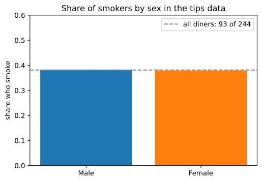
38.2% of men and 37.9% of women in the data smoke, both close to the overall 38.1%. That is what "independent" looks like, and why χ² is near 0.
Chi-square test of independence vs goodness of fit
| Test of independence | Goodness of fit | |
|---|---|---|
| Question | Are two categorical variables related? | Does one variable match stated shares? |
| Table | r × c contingency table | One row of k counts |
| Expected count | Row total × column total / N | n × stated share |
| Degrees of freedom | (r − 1)(c − 1) | k − 1 |
| SciPy | chi2_contingency(table, correction=...) | chisquare(f_obs, f_exp) |
Where you use a chi-square test of independence
- Survey analysis: is product preference related to gender, region or age band?
- A/B tests on yes/no outcomes: is buying related to which page design a user saw?
- Feature screening: is a categorical feature related to a categorical target before it goes into a model?
stats.fisher_exact(table). A significant χ² also says nothing about cause, only that the variables are not independent in this data.Related
- Previous: Chi-square goodness-of-fit test
- Next: One-way ANOVA (F-test)
- Reference: scipy.stats.chi2_contingency
- Replace the tips table with
[[30, 20], [25, 25]](gender by product preference, 100 customers) and runchi2_contingencywith and without the correction. - Cross
tips["smoker"]withtips["time"]. Is smoking related to lunch or dinner? - Run
stats.fisher_exact(dataset_table)on the sex by smoker table and compare its p-value with 0.9649.
Every expert started right here.