
Type I and Type II errors
Type I and Type II errors are the two wrong decisions a hypothesis test can make: a Type I error rejects a null hypothesis that is true, and a Type II error fails to reject a null hypothesis that is false.
Last updated: 07 Oct, 2026 · SciPy 1.18
The Significance level, one-tailed and two-tailed tests lesson defined α as the chance of rejecting a true H₀. That is one of two ways a test can go wrong. Keeping both in view is what lets you choose α and the sample size sensibly.
Listing the four outcomes of a test
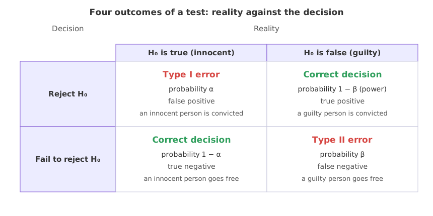
The video keeps the coin: H₀ says the coin is fair, H₁ says it is not. After the experiment there are two sides to compare. The reality check: H₀ is either true or false, though we never see which. The decision: we either reject H₀ or fail to reject it. Crossing the two gives four outcomes:
- Reject H₀ when in reality it is false: a good decision.
- Reject H₀ when in reality it is true: a bad decision, called a Type I error. With H₀ "the person is innocent", this is convicting an innocent person.
- Fail to reject H₀ when in reality it is false: a bad decision, called a Type II error. The person committed the crime and goes free.
- Fail to reject H₀ when in reality it is true: a good decision.
Outcomes 3 and 4 are often worded "accept H₀". The exact wording is "fail to reject H₀": a test that does not reject has not shown that H₀ is true.
Matching the errors to a confusion matrix
Call "reject H₀" (an effect detected) a positive. Then a false positive (FP) is a Type I error and a false negative (FN) is a Type II error; true positives and true negatives are the correct decisions. A cancer screening test that flags a healthy patient makes a Type I error; one that clears a patient who has cancer makes a Type II error. The mapping depends on which class is called positive. The Confusion matrix lesson of the Machine Learning course uses the same four cells for classifiers.
Defining α, β and power
- α = P(Type I error) = P(reject H₀ | H₀ true): the significance level, chosen before the data.
- β = P(Type II error) = P(fail to reject H₀ | H₁ true): it depends on how far the truth is from H₀ and on the sample size.
- Power = 1 − β = P(reject H₀ | H₁ true): the chance the test detects a real effect.
For a fixed sample size, lowering α makes the rejection region smaller, so real effects are missed more often and β rises. Raising n makes the share of heads vary less under both hypotheses, so their distributions overlap less and β falls at the same α. Planning a study means picking α, the smallest effect worth detecting, and the n that gives enough power, often 0.8.
Computing α, β and power for the coin test
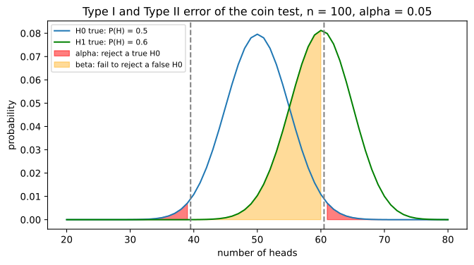
Take the coin test from the hypothesis testing lesson (100 tosses, α = 0.05, reject at 39 or fewer heads or 61 or more) and suppose the coin is in fact biased, landing heads 60% of the time. The Type I rate is the chance of the rejection region under p = 0.5; the power is the chance of the same region under p = 0.6.
A function for the rejection region
import numpy as np
from scipy.stats import binom

def region(n, alpha):
    k = np.arange(n + 1)
    lo = k[binom.cdf(k, n, 0.5) <= alpha / 2].max()    # lower cut under H0: p = 0.5
    hi = k[binom.sf(k - 1, n, 0.5) <= alpha / 2].min()  # upper cut
    return int(lo), int(hi)
The chance of rejecting for any true P(H)
def reject_prob(n, alpha, p):
    lo, hi = region(n, alpha)
    return binom.cdf(lo, n, p) + binom.sf(hi - 1, n, p)  # P(X <= lo) + P(X >= hi)
With p = 0.5 this gives the Type I error rate; with p = 0.6 it gives the power, and β = 1 − power.
for n, alpha in ((100, 0.05), (100, 0.01), (200, 0.05), (400, 0.05)):
    a = reject_prob(n, alpha, 0.5)        # Type I error rate: the coin is fair
    power = reject_prob(n, alpha, 0.6)    # the coin lands heads 60% of the time
    print(f"n = {n}, alpha = {alpha}: region {region(n, alpha)}, "
f"Type I rate {a:.4f}, beta {1 - power:.4f}, power {power:.4f}")n = 100, alpha = 0.05: region (39, 61), Type I rate 0.0352, beta 0.5379, power 0.4621 n = 100, alpha = 0.01: region (36, 64), Type I rate 0.0066, beta 0.7614, power 0.2386 n = 200, alpha = 0.05: region (85, 115), Type I rate 0.0400, beta 0.2132, power 0.7868 n = 400, alpha = 0.05: region (179, 221), Type I rate 0.0402, beta 0.0238, power 0.9762
What the error rates show
- n = 100, α = 0.05: the Type I rate is 0.0352 and the power against p = 0.6 is only 0.4621, so β = 0.5379. More often than not, 100 tosses miss a coin that lands heads 60% of the time.
- A stricter α = 0.01 widens the non-rejection range to 37 to 63: the Type I rate drops to 0.0066, but β rises to 0.7614. Lowering α raises β.
- More tosses: at α = 0.05, power grows to 0.7868 with 200 tosses and 0.9762 with 400. A larger sample lowers β without touching α.
Checking the error rates by simulation
The same numbers come out of repeating the experiment: 10,000 runs of 100 tosses with a fair coin, then 10,000 with the biased one, counting how often the test rejects.
rng = np.random.default_rng(42)
lo, hi = region(100, 0.05)
for p in (0.5, 0.6):
    heads = rng.binomial(100, p, size=10000)          # 10,000 runs of 100 tosses
    rejected = np.mean((heads <= lo) | (heads >= hi))
    print(f"true P(H) = {p}: H0 rejected in {rejected:.4f} of the runs")
print("20 tests of true nulls at alpha 0.05, P(at least one Type I error) =", round(1 - 0.95 ** 20, 3))true P(H) = 0.5: H0 rejected in 0.0393 of the runs true P(H) = 0.6: H0 rejected in 0.4602 of the runs 20 tests of true nulls at alpha 0.05, P(at least one Type I error) = 0.642
- With the fair coin, 0.0393 of the runs reject H₀, near the exact Type I rate 0.0352 (a simulation carries its own sampling noise). Every one of those rejections is a Type I error.
- With the biased coin, 0.4602 of the runs reject, close to the exact power 0.4621; the other runs are Type II errors.
- Twenty tests of true null hypotheses at α = 0.05 give at least one Type I error with probability 0.642. Running many tests and reporting the significant ones inflates false alarms.
import numpy as np
import matplotlib.pyplot as plt
from scipy.stats import binom

k = np.arange(20, 81)
null, alt = binom.pmf(k, 100, 0.5), binom.pmf(k, 100, 0.6)
reject = (k <= 39) | (k >= 61)                 # the alpha = 0.05 region for n = 100
plt.figure(figsize=(8, 4))
plt.plot(k, null, color="tab:blue", label="H0 true: P(H) = 0.5")
plt.plot(k, alt, color="green", label="H1 true: P(H) = 0.6")
plt.fill_between(k, null, where=reject, color="red", alpha=0.5, label="alpha: reject a true H0")
plt.fill_between(k, alt, where=~reject, color="orange", alpha=0.4, label="beta: fail to reject a false H0")
plt.axvline(39.5, color="grey", linestyle="--")
plt.axvline(60.5, color="grey", linestyle="--")
plt.title("Type I and Type II error of the coin test, n = 100, alpha = 0.05")
plt.xlabel("number of heads")
plt.ylabel("probability")
plt.legend(loc="upper left", fontsize=8)
plt.show()
print("alpha =", round(null[reject].sum(), 4), " beta =", round(alt[~reject].sum(), 4))alpha = 0.0352 beta = 0.5379
Type I error vs Type II error
| Type I error | Type II error | |
|---|---|---|
| Decision | Reject H₀ | Fail to reject H₀ |
| Reality | H₀ is true | H₀ is false |
| Probability | α | β |
| Also called | False positive | False negative |
| Court example | An innocent person is convicted | A guilty person goes free |
| Made smaller by | A smaller α | A larger n, a larger α, a bigger true effect |
Where you use Type I and Type II errors
- Medical screening: a Type II error (a missed disease) is often worse than a Type I error (a follow-up test), so screening favours high power.
- Spam filters: a Type I error sends a real email to spam, so the filter is tuned to keep that rate low.
- A/B test planning: choose α, the smallest lift worth detecting, and the sample size that gives power 0.8 before the test starts.
Related
- Previous: Significance level, one-tailed and two-tailed tests
- Next: One-sample z-test
- Reference: scipy.stats.binom
- Compute the power against a coin with P(H) = 0.7:
reject_prob(100, 0.05, 0.7). Why is it so much higher? - Find the smallest n in
range(100, 400, 20)withreject_prob(n, 0.05, 0.6) >= 0.8. - In the simulation, change
size=10000tosize=1000. How much do the rejection shares move?
This is what real progress feels like.