
Point estimates and standard error
A point estimate is a single number computed from a sample, such as the sample mean x̄, that estimates an unknown population parameter, such as the population mean μ.
Last updated: 07 Oct, 2026 · SciPy 1.18
The Central limit theorem lesson showed that sample means pile up in a bell around μ. Inference starts from that fact: one sample gives one estimate, and the standard error says how far such an estimate typically lands from the truth.
Estimating a population mean with x̄
A point estimate is the value of a statistic that estimates the value of a parameter. Two words carry the idea. A statistic is a number computed from a sample (x̄, s, p̂). A parameter is the matching number for the whole population (μ, σ, p), and it is usually unknown.
Inferential statistics works in one direction: from a sample to the population. With the sample mean x̄ we estimate the population mean μ. The video's example: a sample gives x̄ = 2.9 while the population mean is μ = 3. The estimate may land a little below μ, a little above it, or on it. A different sample would give a different x̄, as the board notes' other samples show (2.8, 2.5, 3.5). The Population and sample lesson set up this vocabulary.
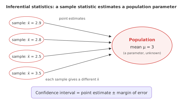
Because a point estimate almost never equals the parameter exactly, it is reported with a range around it. That range is the confidence interval, built as:
The margin of error is a multiple of the standard error, the subject of the rest of this page.
Common point estimates and their parameters
| Parameter (population) | Point estimate (sample) | Note |
|---|---|---|
| Mean μ | Sample mean x̄ = Σxᵢ / n | Unbiased: its average over all samples is μ |
| Variance σ² | Sample variance s² = Σ(xᵢ − x̄)² / (n − 1) | Unbiased because of the n − 1 divisor |
| Standard deviation σ | Sample SD s | Slightly biased low, still the usual choice |
| Proportion p | Sample proportion p̂ = x / n | Unbiased: its average over all samples is p |
An estimator is unbiased when its average over all possible samples equals the parameter. The Sample variance and why n − 1 lesson shows why s² divides by n − 1 for exactly this reason.
Measuring the spread of x̄ with the standard error
The standard error (SE) of a statistic is the standard deviation of its sampling distribution: how much the statistic varies from one sample to the next. For the sample mean of n independent observations from a population with standard deviation σ:
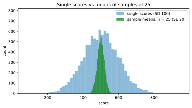
The CAT example from the video has σ = 100 and n = 25, so SE = 100 / √25 = 100 / 5 = 20. Single scores spread with an SD of 100; means of 25 scores spread with an SD of only 20. Quadrupling n halves the SE, because √n grows from 5 to 10.
Simulating the standard error
The code draws 10,000 samples from a normal population with μ = 500 and σ = 100, takes the mean of each, and compares the spread of those means with σ/√n, first for n = 25 and then for n = 100.
import numpy as np
import matplotlib.pyplot as plt

rng = np.random.default_rng(42)
mu, sigma = 500, 100                              # a population of test scores

for n in (25, 100):
    means = rng.normal(mu, sigma, size=(10000, n)).mean(axis=1)   # 10,000 samples, one x̄ each
    print(f"n = {n:3}: average x̄ {means.mean():.2f}, SD of the x̄ values {means.std(ddof=1):.2f}, "
          f"sigma/sqrt(n) {sigma / np.sqrt(n):.2f}")

scores = rng.normal(mu, sigma, size=10000)                         # single scores
means25 = rng.normal(mu, sigma, size=(10000, 25)).mean(axis=1)     # means of 25 scores
plt.figure(figsize=(8, 4))
plt.hist(scores, bins=60, alpha=0.5, label="single scores (SD 100)")
plt.hist(means25, bins=60, alpha=0.7, color="green", label="sample means, n = 25 (SE 20)")
plt.title("Single scores vs means of samples of 25")
plt.xlabel("score")
plt.ylabel("count")
plt.ylim(0, 820)
plt.legend(loc="upper right")
plt.show()n = 25: average x̄ 500.01, SD of the x̄ values 20.03, sigma/sqrt(n) 20.00 n = 100: average x̄ 500.10, SD of the x̄ values 9.84, sigma/sqrt(n) 10.00
What the simulated means show
- The average x̄ sits on μ (500.01 for n = 25, 500.10 for n = 100): x̄ is an unbiased estimate of the population mean.
- The SD of the x̄ values matches σ/√n: 20.03 against 20 for n = 25, and 9.84 against 10 for n = 100. Ten thousand samples are a simulation, so the match is close rather than exact.
- The histogram of means is much narrower than the histogram of single scores, though both are centred at 500. The standard error describes the green one.
Computing the standard error of one sample
In practice there is one sample and σ is unknown, so the SE is estimated as s/√n, with s the sample standard deviation (divisor n − 1). SciPy's stats.sem does the same computation; its ddof parameter defaults to 1. The data is the ages sample from the t-test notebook in the video's materials.
import numpy as np
from scipy import stats

ages = [18, 10, 24, 10, 35, 55, 10, 70, 18, 28]   # the ages sample of the t-test notebook
s = np.std(ages, ddof=1)                          # sample SD, divisor n - 1
print("x̄ =", np.mean(ages), "  s =", round(s, 3), "  n =", len(ages))
print("SE by hand, s/sqrt(n) =", round(s / np.sqrt(len(ages)), 3))
print("stats.sem(ages) =", round(stats.sem(ages), 3))x̄ = 27.8 s = 20.357 n = 10 SE by hand, s/sqrt(n) = 6.437 stats.sem(ages) = 6.437
- The sample mean is 27.8 and the sample SD is 20.357: the ages are widely spread.
- The estimated SE is 6.437, by hand and with
stats.sem: a mean of 10 ages is far less spread out than a single age.
Standard deviation vs standard error
| Standard deviation (σ or s) | Standard error (σ/√n or s/√n) | |
|---|---|---|
| Describes | The spread of individual values | The spread of a statistic, such as x̄, across samples |
| Changes with n | No: it is a property of the data | Yes: it shrinks as 1/√n |
| CAT example | 100 (σ) or 80 (s) | 100/√25 = 20 or 80/√25 = 16 |
| Used for | Describing the data, z-scores of single values | Confidence intervals and test statistics |
Where you use the standard error
- Confidence intervals: the margin of error is a critical value times the SE, as in x̄ ± 1.96 σ/√n.
- Test statistics: z = (x̄ − μ₀)/(σ/√n) measures a difference in units of standard error.
- Error bars on a chart of group means, where the label must say whether the bars show the SD or the SE.
Related
- Previous: Central limit theorem
- Next: Confidence intervals
- Reference: scipy.stats.sem
- Add
400to the loop,for n in (25, 100, 400). Is the SD of the means close to 100/√400 = 5? - Change
sigmato 50. What happens to every standard error? - Run
stats.sem(ages, ddof=0). Why is it a little smaller than 6.437?
This is what real progress feels like.