
Skewness and kurtosis
Skewness is a measure of the asymmetry of a distribution, and kurtosis is a measure of how heavy its tails are compared with a normal distribution.
Last updated: 07 Oct, 2026 · SciPy 1.18
Centre (Mean, median and mode) and spread (Variance and standard deviation) do not describe shape. Two datasets with the same mean and standard deviation can lean in opposite directions, or differ in how often extreme values turn up. Skewness and kurtosis put a number on each of those two features.
Reading skew from the mean, median and mode
In a right-skewed (positively skewed) distribution the right tail is longer: most values are small and a few are large. The large values pull the mean to the right of the median, and the mode, the peak, sits to the left of both, so mean > median > mode. A left-skewed distribution is the mirror image, mean < median < mode, and in a symmetric one with a single peak all three are equal.
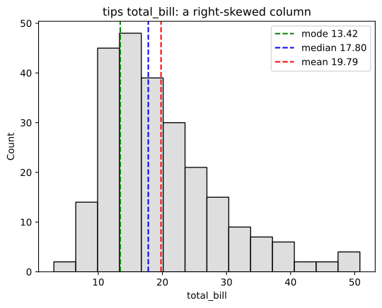
The tips dataset that the video loads in its Colab session shows it. Its total_bill column has a mean of 19.79, a median of 17.795 and a mode of 13.42 (the most repeated bill, three times): mean > median > mode, with a long right tail in its histogram. A mean above the median can come from a few outliers or from a long skewed tail; the histogram and the skewness tell the two apart.
The order is a rule of thumb for smooth distributions with one peak. Discrete data and data with several peaks can break it, so compute the skewness instead of relying on the order alone.
Measuring skewness
The usual measure is the Fisher-Pearson coefficient: the average cubed deviation divided by the standard deviation cubed. Cubing keeps the sign, so a long right tail gives a positive number and a long left tail a negative one; a symmetric distribution scores 0.
A common rule of thumb reads a skewness between −0.5 and 0.5 as close to symmetric, between 0.5 and 1 in size as moderately skewed, and beyond 1 as highly skewed. The tips bills, at 1.13, are highly right-skewed.
Measuring kurtosis
Kurtosis measures the tailedness of a distribution: how much of its spread comes from rare values far from the mean. Subtracting 3 makes a normal distribution score 0, and that version is called excess kurtosis. Positive excess kurtosis means heavier tails than a normal, so extreme values turn up more often; negative means lighter tails. Kurtosis is about the tails, not about how sharp the peak looks.
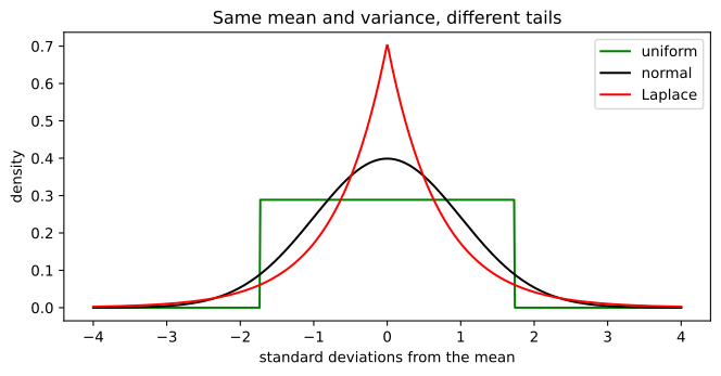
Three distributions with the same mean 0 and variance 1 show the range. A uniform distribution has excess kurtosis −1.2 and never goes beyond 3 standard deviations. A normal distribution has 0 and lands beyond 3 standard deviations 0.27% of the time. A Laplace distribution has 3 and lands there 1.44% of the time, more than five times as often.
Choosing the median when one value pulls the mean
The Q&A notes' page-load use case logs a website's load times in seconds. Day 1 is 3, 2.5, 2.8, 3.1 and 15, where 15 seconds was a server glitch. The glitch lifts the day's mean from 2.85 to 5.28, while the median is 3.0. Over the fifteen loads of days 1 to 3 the mean is 3.57 against a median of 2.8, with a skewness of 3.45 and an excess kurtosis of 9.98. To fill a missing load time, or to report a typical one, the median is the right choice here.
A log transform pulls in a long right tail, and is the usual fix for skewed positive data such as incomes or prices (Log-normal distribution); ln 3 = 1.0986, for example. It does not fix a single glitch: the skewness of the log load times is still 3.33, because 15 seconds stays far from the rest. A value like that needs a decision of its own (Outlier detection with IQR and z-score).
Computing skewness and kurtosis in Python
SciPy's skew and kurtosis
Both default to bias=True, the plain moment formulas above. kurtosis returns excess kurtosis by default (fisher=True); fisher=False adds the 3 back, so a normal scores 3.
from scipy import stats

stats.skew(x)                     # g1, the moment formula
stats.kurtosis(x)                 # excess kurtosis g2 (normal = 0)
stats.kurtosis(x, fisher=False)   # kurtosis with the 3 kept (normal = 3)
pandas' skew and kurt
pandas applies a small-sample correction, the same as SciPy with bias=False, so its numbers differ slightly from SciPy's defaults on the same data. Both report excess kurtosis.
s.skew()     # adjusted Fisher-Pearson skewness
s.kurt()     # adjusted excess kurtosis
Drawing the three shapes
import numpy as np
import matplotlib.pyplot as plt
from scipy import stats

a = 2
right = stats.gamma(a)                         # a right-skewed distribution
mode, median, mean = a - 1, right.median(), right.mean()   # a gamma peaks at a - 1
print("mode:", mode, " median:", round(median, 3), " mean:", mean)
print("skewness:", round(float(right.stats(moments="s")), 3))

x = np.linspace(0, right.ppf(0.999), 400)
top = x.max()
fig, axes = plt.subplots(1, 3, figsize=(10, 3), sharey=True)
axes[0].plot(top - x, right.pdf(x), color="black")              # mirror image: left-skewed
axes[1].plot(x, stats.norm(top / 2, top / 7).pdf(x), color="black")
axes[2].plot(x, right.pdf(x), color="black")
for value, color, name in [(mode, "green", "mode"), (median, "blue", "median"), (mean, "red", "mean")]:
    axes[0].axvline(top - value, color=color, linestyle="--")
    axes[2].axvline(value, color=color, linestyle="--", label=name)
axes[1].axvline(top / 2, color="grey", linestyle="--", label="mean = median = mode")
for ax, title in zip(axes, ["Left-skewed", "Symmetric", "Right-skewed"]):
    ax.set_title(title)
    ax.set_xticks([])
axes[1].legend(loc="upper right", fontsize=8)
axes[2].legend()
plt.show()mode: 1 median: 1.678 mean: 2.0 skewness: 1.414
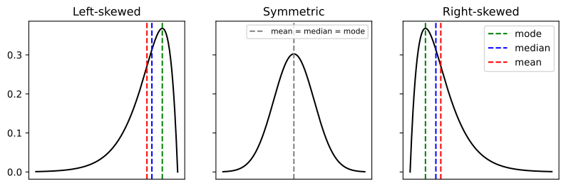
The right-skewed curve is a gamma distribution with shape 2: its mode is 1, its median 1.678 and its mean 2.0, in that order, and its skewness is 1.414. The left-skewed curve is its mirror image.
Comparing the tails of three distributions
import numpy as np
import matplotlib.pyplot as plt
from scipy import stats

shapes = {"uniform": stats.uniform(-np.sqrt(3), 2 * np.sqrt(3)),
          "normal": stats.norm(0, 1),
          "Laplace": stats.laplace(0, 1 / np.sqrt(2))}
for name, dist in shapes.items():
    var, kurt = dist.stats(moments="vk")
    print(f"{name:8} variance={float(var):.2f}  excess kurtosis={float(kurt):5.2f}"
          f"  P(|x| > 3)={2 * dist.sf(3):.4f}")

x = np.linspace(-4, 4, 800)
plt.figure(figsize=(8, 3.6))
for (name, dist), color in zip(shapes.items(), ["green", "black", "red"]):
    plt.plot(x, dist.pdf(x), color=color, label=name)
plt.xlabel("standard deviations from the mean")
plt.ylabel("density")
plt.title("Same mean and variance, different tails")
plt.legend()
plt.show()uniform variance=1.00 excess kurtosis=-1.20 P(|x| > 3)=0.0000 normal variance=1.00 excess kurtosis= 0.00 P(|x| > 3)=0.0027 Laplace variance=1.00 excess kurtosis= 3.00 P(|x| > 3)=0.0144
Measuring the tips bills
import statistics
import numpy as np
import seaborn as sns
import matplotlib.pyplot as plt
from scipy import stats

df = sns.load_dataset("tips")
bill = df["total_bill"]
print("mean:", round(np.mean(bill), 2), " median:", np.median(bill), " mode:", statistics.mode(bill))
print("skewness  scipy:", round(stats.skew(bill), 3), " pandas:", round(bill.skew(), 3))
print("excess kurtosis  scipy:", round(stats.kurtosis(bill), 3), " pandas:", round(bill.kurt(), 3))

sns.histplot(bill, color="lightgrey")
plt.axvline(statistics.mode(bill), color="green", linestyle="--", label="mode 13.42")
plt.axvline(np.median(bill), color="blue", linestyle="--", label="median 17.80")
plt.axvline(np.mean(bill), color="red", linestyle="--", label="mean 19.79")
plt.title("tips total_bill: a right-skewed column")
plt.legend()
plt.show()mean: 19.79 median: 17.795 mode: 13.42 skewness scipy: 1.126 pandas: 1.133 excess kurtosis scipy: 1.169 pandas: 1.218
What the tips run shows
- Mean 19.79, median 17.795, mode 13.42: the order of a right-skewed column, matching the video's Colab output.
- Skewness 1.126 with SciPy and 1.133 with pandas: the same data, two formulas, both highly right-skewed.
- Excess kurtosis 1.169 with SciPy and 1.218 with pandas: heavier tails than a normal, from the few large bills.
Measuring the page-load times
import numpy as np
from scipy import stats

day1 = np.array([3, 2.5, 2.8, 3.1, 15])            # 15 s was a server glitch
print("day 1 mean:", round(day1.mean(), 2), " without 15:", day1[:4].mean(), " median:", np.median(day1))

loads = np.array([3, 2.5, 2.8, 3.1, 15, 2.6, 2.5, 2.7, 2.9, 2.8, 2.7, 2.8, 2.6, 2.5, 3])
print("15 loads  mean:", round(loads.mean(), 2), " median:", np.median(loads))
print("skewness:", round(stats.skew(loads), 2), " excess kurtosis:", round(stats.kurtosis(loads), 2))
print("ln(3) =", round(np.log(3), 4), " skewness of ln(loads):", round(stats.skew(np.log(loads)), 2))day 1 mean: 5.28 without 15: 2.85 median: 3.0 15 loads mean: 3.57 median: 2.8 skewness: 3.45 excess kurtosis: 9.98 ln(3) = 1.0986 skewness of ln(loads): 3.33
What the page-load run shows
- Day 1's mean is 5.28 with the glitch and 2.85 without it; its median is 3.0 either way.
- Over fifteen loads the mean is 3.57 and the median 2.8, with skewness 3.45 and excess kurtosis 9.98, both caused by one value.
- The log transform moves the skewness only to 3.33: one glitch is an outlier, not a skewed shape.
Skewness vs kurtosis
| Skewness | Kurtosis (excess) | |
|---|---|---|
| Describes | asymmetry: which tail is longer | tailedness: how heavy both tails are |
| Based on | cubed deviations (m₃) | fourth-power deviations (m₄) |
| Normal distribution | 0 | 0 |
| Sign | + right tail longer, − left tail longer | + heavier tails, − lighter tails |
| Tips total_bill | 1.126 | 1.169 |
Where you use skewness and kurtosis
- Choosing the centre: a highly skewed column gets the median, both for reporting and for filling missing values.
- Deciding on a log transform for incomes, prices or durations before fitting a linear model.
- Finance and risk: returns with high kurtosis produce extreme days more often than a normal model predicts.
Related
- Previous: Range, MAD and coefficient of variation
- Next: Percentiles and percentile rank
- See also: Normality tests (Q-Q plot and Shapiro-Wilk)
- Remove the 15 from
loadsand compute the skewness again. - Change
a = 2toa = 20in the gamma example and watch the mean, median and mode move closer together. - Compute
stats.skew(df['tip'])for the tips column and compare it withtotal_bill.
Every expert started right here.