
Variance and standard deviation
Variance is a measure of dispersion that averages the squared distances of the values from their mean, and the standard deviation is its square root, a typical distance from the mean in the data's own units.
Last updated: 07 Oct, 2026 · SciPy 1.18
Mean, median and mode gives one number for the centre of the data. Two datasets can share that centre and still look nothing alike, so a second number is needed: how spread out the values are.
Comparing two datasets with the same mean
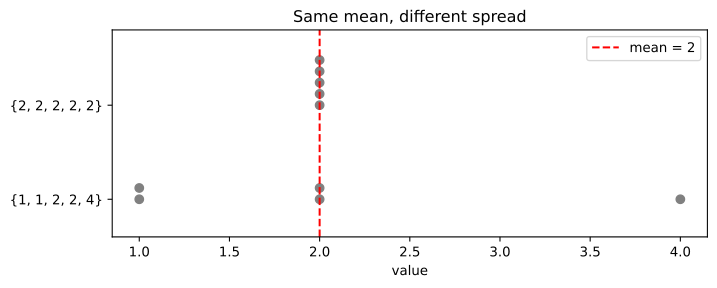
Dispersion means spread: how well the values are spread around the mean. The datasets {1, 1, 2, 2, 4} and {2, 2, 2, 2, 2} both have a mean of 10/5 = 2. In the second every value is the mean and there is no spread at all; the first has values on both sides. The mean cannot tell them apart. Variance and standard deviation can: the first dataset has a population variance of 1.2 and the second 0.
Writing the population and sample variance
Each deviation x − μ is squared, so values below the mean and values above it both add to the spread instead of cancelling out. Why the sample formula divides by n − 1 is a common interview question; Sample variance and why n − 1 answers it.
Working the variance of 1, 2, 2, 3, 4, 5 by hand
The video's example has six values. Their mean is μ = 17/6 = 2.83. The table takes each value's deviation from the mean, squares it and adds the squares:
| x | x − μ | (x − μ)² |
|---|---|---|
| 1 | −1.83 | 3.36 |
| 2 | −0.83 | 0.69 |
| 2 | −0.83 | 0.69 |
| 3 | 0.17 | 0.03 |
| 4 | 1.17 | 1.36 |
| 5 | 2.17 | 4.69 |
| Sum | 0 | 10.83 |
The video treats the six values as the whole population and divides by N = 6: σ² = 10.83/6 = 1.81. Treated as a sample, the same sum is divided by n − 1 = 5: s² = 10.83/5 = 2.17. With six values the two answers differ by 20%. Which one is right depends on the data: divide by N when the values are the entire population, and by n − 1 when they are a sample from something larger.
Taking the square root to get the standard deviation
Variance is in squared units: if the values are in kilograms, the variance is in kilograms squared. The standard deviation is the square root of the variance, which brings the spread back to the data's own units. That is why it is the number usually reported.
A larger variance means the values sit farther from the mean, with fewer of them close to it. Drawn as a curve, data with a small standard deviation gives a tall, narrow peak, and data with a large one gives a low, wide curve.
Measuring distance from the mean in standard deviations
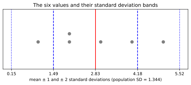
The standard deviation also works as a unit of distance. With the mean 2.833 and the population standard deviation 1.344, one standard deviation to the right is 2.833 + 1.344 = 4.18 and one to the left is 2.833 − 1.344 = 1.49. Two standard deviations to the right is 2.833 + 2 × 1.344 = 5.52. The value 5 lies (5 − 2.833)/1.344 = 1.61 standard deviations above the mean. A distance measured in standard deviations is the idea behind the Z-score and the standard normal distribution lesson.
Four of the six values lie within one standard deviation of the mean. The well-known 68%, 95% and 99.7% for one, two and three standard deviations hold for data that follow a normal distribution (Empirical rule (68-95-99.7)), not for any set of numbers.
Computing variance and standard deviation in Python
NumPy divides by N unless you set ddof=1
ddof means delta degrees of freedom: the divisor is N − ddof. NumPy's default is ddof=0, the population formula.
import numpy as np

x = np.array([1, 2, 2, 3, 4, 5])
np.var(x)             # population variance, divides by N
np.var(x, ddof=1)     # sample variance, divides by n - 1
np.std(x, ddof=1)     # sample standard deviation
pandas divides by n − 1 by default
import pandas as pd

s = pd.Series([1, 2, 2, 3, 4, 5])
s.var()               # sample variance, ddof=1 is the default
s.std(ddof=0)         # population standard deviation
The statistics module names both
import statistics

statistics.pvariance([1, 2, 2, 3, 4, 5])   # population variance
statistics.variance([1, 2, 2, 3, 4, 5])    # sample variance
statistics.stdev([1, 2, 2, 3, 4, 5])       # sample standard deviation
Same mean, different spread
import numpy as np
import matplotlib.pyplot as plt

a = [1, 1, 2, 2, 4]
b = [2, 2, 2, 2, 2]
print("means:    ", np.mean(a), np.mean(b))
print("variances:", np.var(a), np.var(b))

fig, ax = plt.subplots(figsize=(8, 2.8))
for row, data in enumerate([a, b]):
    seen = {}
    for v in data:
        seen[v] = seen.get(v, 0) + 1
        ax.scatter(v, row + 0.12 * (seen[v] - 1), color="grey", s=40)
ax.axvline(2, color="red", linestyle="--", label="mean = 2")
ax.set_yticks([0, 1], ["{1, 1, 2, 2, 4}", "{2, 2, 2, 2, 2}"])
ax.set_ylim(-0.4, 1.8)
ax.set_xlabel("value")
ax.set_title("Same mean, different spread")
ax.legend()
plt.show()means: 2.0 2.0 variances: 1.2 0.0
Working the six values in code
import numpy as np
import pandas as pd
import matplotlib.pyplot as plt

x = np.array([1, 2, 2, 3, 4, 5])
mu = x.mean()
print("mean:", round(mu, 4))
print("deviations x - mean:", np.round(x - mu, 4))
print("squared:", np.round((x - mu) ** 2, 4), " sum:", round(((x - mu) ** 2).sum(), 4))
print("np.var  ddof=0:", round(np.var(x), 4), "  ddof=1:", round(np.var(x, ddof=1), 4))
print("np.std  ddof=0:", round(np.std(x), 4), "  ddof=1:", round(np.std(x, ddof=1), 4))
print("pandas var, std:", round(pd.Series(x).var(), 4), round(pd.Series(x).std(), 4))

sd = np.std(x)
print("mean -2, -1, +1, +2 SD:", [float(round(mu + k * sd, 2)) for k in (-2, -1, 1, 2)])
print("5 is", round((5 - mu) / sd, 2), "standard deviations above the mean")

fig, ax = plt.subplots(figsize=(8, 2.6))
ax.scatter(x, [0, 0, 0.15, 0, 0, 0], color="grey", s=50, zorder=3)
ax.axvline(mu, color="red", label="mean")
for k in (1, 2):
    for side in (-1, 1):
        ax.axvline(mu + side * k * sd, color="blue", linestyle="--" if k == 1 else ":")
ax.set_xticks([round(mu + k * sd, 2) for k in (-2, -1, 0, 1, 2)])
ax.set_yticks([])
ax.set_ylim(-0.5, 0.6)
ax.set_xlabel("mean ± 1 and ± 2 standard deviations (population SD = 1.344)")
ax.set_title("The six values and their standard deviation bands")
plt.show()mean: 2.8333 deviations x - mean: [-1.8333 -0.8333 -0.8333 0.1667 1.1667 2.1667] squared: [3.3611 0.6944 0.6944 0.0278 1.3611 4.6944] sum: 10.8333 np.var ddof=0: 1.8056 ddof=1: 2.1667 np.std ddof=0: 1.3437 ddof=1: 1.472 pandas var, std: 2.1667 1.472 mean -2, -1, +1, +2 SD: [0.15, 1.49, 4.18, 5.52] 5 is 1.61 standard deviations above the mean
What the variance run shows
- The two sets both have a mean of 2.0, with variances 1.2 and 0.0.
- The deviations add up to zero, and the squares add up to 10.8333.
- NumPy's default gives the population variance 1.8056 and standard deviation 1.3437;
ddof=1gives the sample values 2.1667 and 1.472. - pandas prints 2.1667 and 1.472 with no arguments, because its default is the sample formula.
- One standard deviation either side of the mean runs from 1.49 to 4.18, two from 0.15 to 5.52, and 5 is 1.61 standard deviations above the mean.
Variance vs standard deviation
| Variance | Standard deviation | |
|---|---|---|
| Formula | mean squared deviation | square root of the variance |
| Units | squared (kg²) | the data's own (kg) |
| Value for 1, 2, 2, 3, 4, 5 | 1.806 (÷N), 2.167 (÷ n − 1) | 1.344 (÷N), 1.472 (÷ n − 1) |
| Used for | the maths: variances of independent variables add | reporting spread, z-scores, error bars |
Where you use variance and standard deviation
- Comparing consistency: two machines filling 500 g bags with the same mean weight; the one with the smaller standard deviation fills more evenly.
- Scaling features for machine learning: standardization divides each feature by its standard deviation (Standardization and normalization).
- Risk: the standard deviation of an investment's returns is the usual measure of how volatile it is.
np.std(x) and pd.Series(x).std() give different numbers for the same data, 1.344 and 1.472 here, because NumPy divides by N and pandas by n − 1. Set ddof yourself whenever the result matters.Related
- Previous: Mean, median and mode
- Next: Sample variance and why n − 1
- See also: Empirical rule (68-95-99.7)
- Replace 5 with 50 in
xand see how much the variance and the standard deviation grow. - Pass the NumPy array
xtostatistics.pvarianceinstead of a list and read the result: the module keeps NumPy's integer type and prints 1. - Compute the variance of {2, 2, 2, 2, 2} with
ddof=1and check that it is still 0.
You understood something today that you didn't yesterday.