
Normal (Gaussian) distribution
The normal distribution (also called the Gaussian distribution) is a continuous probability distribution with a symmetric, bell-shaped curve, fixed completely by two numbers: the mean μ, which sets the centre, and the standard deviation σ, which sets the spread.
Last updated: 07 Oct, 2026 · SciPy 1.18
The z-score rule in Outlier detection with IQR and z-score flagged values more than three standard deviations from the mean. That cut-off comes from one curve, the normal distribution, which much of statistics is built on.
Reading the bell curve
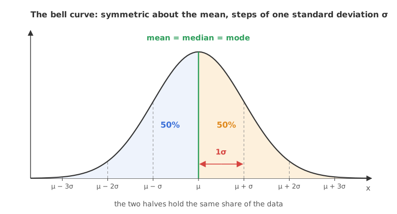
The video draws the normal distribution as a bell curve. Its centre line is the mean, and for a normal distribution the median and the mode sit on the same line. The curve is symmetric: the part to the right of the centre is a mirror image of the part to the left, so each half holds the same amount of the data, 50%.
From the centre the video steps out one standard deviation at a time: one, two and three standard deviations to the right, and the same to the left. With μ for the mean and σ for the standard deviation, the steps are labelled μ − 3σ, μ − 2σ, μ − σ, μ, μ + σ, μ + 2σ and μ + 3σ. How much of the data falls between these steps is the subject of Empirical rule (68-95-99.7).
Writing the normal pdf
The bell curve of the normal distribution has an exact formula, its probability density function (pdf):
The short way to write it is X ~ N(μ, σ²): X is normally distributed with mean μ and variance σ². scipy names the two numbers loc and scale, and scale is the standard deviation σ, not the variance.
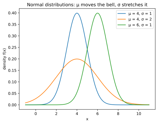
- μ moves the curve. A different mean slides the whole bell left or right without changing its shape.
- σ stretches the curve. A larger standard deviation makes the bell lower and wider, a smaller one taller and narrower. The peak height is 1/(σ√(2π)), 0.3989 when σ = 1.
- The total area is 1. The curve never touches the axis, but the area under all of it is exactly 1, the total probability.
- Mean, median and mode are equal. Symmetry puts all three at μ, which is why the centre line carries all three names.
Finding probabilities as areas
The normal distribution is continuous: X can take any value, 4.5 or 4.5001 or 4.50001. A probability is the area under the curve over an interval, and the cumulative distribution function (cdf) F(x) = P(X ≤ x) gives those areas:
Two facts follow. The probability of one exact value is 0, because a single point has no width: P(X = 4.5) = 0, and so P(X < 4.5) = P(X ≤ 4.5). And f(x) is a density, not a probability, so it can be larger than 1: a normal curve with σ = 0.1 peaks at 3.989. Probability density function (PDF) and KDE draws the same line between density and probability.
Computing the normal distribution with scipy.stats.norm
A normal distribution object
norm(loc=4, scale=1) builds the video's distribution, mean 4 and standard deviation 1. .pdf gives the height of the curve and .cdf the area to the left of a point.
from scipy.stats import norm

X = norm(loc=4, scale=1)      # mean 4, standard deviation 1
X.pdf(4.5)                    # height of the curve at 4.5 (a density)
X.cdf(5) - X.cdf(3)           # area between 3 and 5 (a probability)
The pdf formula by hand
The same curve written straight from the formula, to check that scipy computes what the formula says:
import numpy as np

def normal_pdf(x, mu, sigma):
return np.exp(-(x - mu) ** 2 / (2 * sigma ** 2)) / (sigma * np.sqrt(2 * np.pi))from scipy.integrate import quad
X = norm(loc=4, scale=1)
for x in [3.75, 4, 4.5, 4.75]:
print(f"f({x}) = {X.pdf(x):.4f} by hand {normal_pdf(x, 4, 1):.4f}")
print("P(3 <= X <= 5) =", round(X.cdf(5) - X.cdf(3), 4))
print("P(X = 4.5) =", X.cdf(4.5) - X.cdf(4.5))
area, _ = quad(X.pdf, -np.inf, np.inf)
print("total area =", round(area, 4))
print("mean, median =", X.mean(), X.median())
print("peak of N(4, 0.1^2) =", round(norm.pdf(4, loc=4, scale=0.1), 3))f(3.75) = 0.3867 by hand 0.3867 f(4) = 0.3989 by hand 0.3989 f(4.5) = 0.3521 by hand 0.3521 f(4.75) = 0.3011 by hand 0.3011 P(3 <= X <= 5) = 0.6827 P(X = 4.5) = 0.0 total area = 1.0 mean, median = 4.0 4.0 peak of N(4, 0.1^2) = 3.989
Plotting three normal curves
import numpy as np
import matplotlib.pyplot as plt
from scipy.stats import norm

x = np.linspace(-1, 11, 500)
params = [(4, 1), (4, 2), (6, 1)]
for mu, sigma in params:
    plt.plot(x, norm.pdf(x, loc=mu, scale=sigma), label=f"μ = {mu}, σ = {sigma}")
plt.title("Normal distributions: μ moves the bell, σ stretches it")
plt.xlabel("x")
plt.ylabel("density f(x)")
plt.legend()
plt.show()
for mu, sigma in params:
print(f"N({mu}, {sigma}^2): peak {norm.pdf(mu, mu, sigma):.4f} at x = {mu}")N(4, 1^2): peak 0.3989 at x = 4 N(4, 2^2): peak 0.1995 at x = 4 N(6, 1^2): peak 0.3989 at x = 6
What the normal values show
- f(4) = 0.3989 is the peak, 1/√(2π), and the formula by hand matches scipy at every point.
- f(4.5) = 0.3521 and f(4.75) = 0.3011: the further from the mean, the lower the curve. These are densities; none of them is the chance of getting that exact value.
- P(3 ≤ X ≤ 5) = 0.6827: the area within one standard deviation of the mean, the 68% of the empirical rule.
- P(X = 4.5) = 0.0: one point has no area.
- The total area is 1.0, and the mean and the median are both 4.0.
- A σ of 0.1 gives a peak of 3.989, a density above 1. In the plot, doubling σ from 1 to 2 halves the peak from 0.3989 to 0.1995, and moving μ from 4 to 6 slides the bell without changing it.
Normal vs skewed distributions
Skewness, from Skewness and kurtosis, is the quickest way to tell the two apart.
| Normal | Right-skewed | |
|---|---|---|
| Shape | Symmetric bell | Long tail to the right |
| Mean, median, mode | All equal, at μ | Pulled apart, usually mean > median > mode |
| Skewness | 0 | Positive |
| Fixed by | μ and σ | Its own parameters |
| 68-95-99.7 rule | Holds | Does not hold |
| Examples | Measurement errors; heights within one group of adults | Incomes, house prices, restaurant bills |
Where you use the normal distribution
- Measurements. Repeated measurement errors, and body measurements such as height within one group of people, are close to normal. Many other variables are not, which is why Normality tests (Q-Q plot and Shapiro-Wilk) matters.
- Sample means. The average of many independent values is close to normal even when the values are not; that is the Central limit theorem.
- Probabilities, tests and intervals. z-scores, the One-sample z-test and Confidence intervals all read their areas off the normal curve.
Related
- Previous: Outlier detection with IQR and z-score
- Next: Empirical rule (68-95-99.7)
- See also: Probability density function (PDF) and KDE
- Reference: scipy.stats.norm
- Change
scale=1toscale=0.5in the first example: the peak doubles to 0.7979 and P(3 ≤ X ≤ 5) grows to 0.9545. - Print
X.cdf(4.5) - X.cdf(4.4999): a slice 0.0001 wide has a probability of about 0.000035, close to 0. - Add
(0, 1)toparamsin the plot: the curve centred at 0 with σ = 1 is the standard normal distribution.
Every expert started right here.