
Conditional probability and Bayes' theorem
Conditional probability is the probability of an event given that another event has happened, written P(A | B); Bayes' theorem turns P(B | A) around into P(A | B).
Last updated: 07 Oct, 2026 · SciPy 1.18
The Multiplication rule and independent events used P(A | Q), the chance of an ace once a queen was out of the deck, and the video names it conditional probability and points ahead to Bayes' theorem and naive Bayes.
Defining conditional probability
Knowing that B happened shrinks the sample space to the outcomes in B. The probability of A is then the share of B that is also A:
Take one card from a deck. Given that it is red, what is the chance it is a heart? Half the 26 red cards are hearts, so P(heart | red) = (13/52) ÷ (26/52) = 1/2. Without the extra information P(heart) = 1/4, so knowing the colour changed the probability: "heart" and "red" are dependent.
Now ask for P(queen | heart). There is one queen among the 13 hearts, so P(queen | heart) = (1/52) ÷ (13/52) = 1/13. That is the same as P(queen) = 4/52 = 1/13, so knowing the suit tells you nothing about the rank: queen and heart are independent, even though they are not mutually exclusive.
The video's second bag has 3 green and 2 red marbles. The first draw is green with probability 3/5. Given that a green came out, 2 red remain among 4, so P(red | green first) = 2/4, and the multiplication rule gives P(green then red) = 3/5 × 2/4 = 3/10.
Deriving Bayes' theorem
The multiplication rule can be written in both directions: P(A and B) = P(A) × P(B | A) = P(B) × P(A | B). Dividing by P(B) gives Bayes' theorem:
- P(A), the prior: the probability of A before seeing B.
- P(B | A), the likelihood: how probable the evidence B is if A is true.
- P(B), the evidence: how probable B is overall.
- P(A | B), the posterior: the updated probability of A after seeing B.
Finding P(B) with the law of total probability
The denominator is often unknown directly. B happens either together with A or together with not A, two mutually exclusive cases, so the addition rule and the multiplication rule give:
Testing for a rare disease
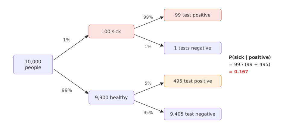
A disease affects 1% of people. A test detects it in 99% of sick people (its sensitivity), and gives a false positive for 5% of healthy people. A person tests positive. What is the chance they are sick?
Only about 1 in 6 positives is sick. Picture 10,000 people: 100 are sick and 99 of them test positive; 9,900 are healthy and 5% of them, 495, also test positive. Of the 594 positives, 99 are sick. The disease is so rare that the false positives from the large healthy group outnumber the true positives.
Computing Bayes' theorem in Python
The function below applies Bayes' theorem with the law of total probability. A simulated population of one million people checks the answer, and a second positive test reuses the first posterior as the new prior.
import numpy as np

def bayes(prior, sensitivity, false_positive_rate):
    """P(sick | positive test) from the prior and the test's error rates."""
    evidence = sensitivity * prior + false_positive_rate * (1 - prior)   # total probability
    return sensitivity * prior / evidence

print("P(sick | +) =", round(bayes(0.01, 0.99, 0.05), 4))

# a simulated population of 1,000,000 people
rng = np.random.default_rng(42)
sick = rng.random(1_000_000) < 0.01
positive = np.where(sick, rng.random(sick.size) < 0.99, rng.random(sick.size) < 0.05)
print("simulated:   ", round(sick[positive].mean(), 4), " positives:", positive.sum())

# a second, independent positive test: yesterday's posterior is today's prior
after_one = bayes(0.01, 0.99, 0.05)
print("after two positives:", round(bayes(after_one, 0.99, 0.05), 4))
for prior in (0.001, 0.01, 0.1, 0.5):
print(f"prevalence {prior:>5}: P(sick | +) = {bayes(prior, 0.99, 0.05):.4f}")P(sick | +) = 0.1667 simulated: 0.1668 positives: 59644 after two positives: 0.7984 prevalence 0.001: P(sick | +) = 0.0194 prevalence 0.01: P(sick | +) = 0.1667 prevalence 0.1: P(sick | +) = 0.6875 prevalence 0.5: P(sick | +) = 0.9519
What the disease numbers mean
- P(sick | +) = 0.1667: a positive result raises the chance from 1% to about 17%, but most positives are still healthy people.
- The simulation agrees: of the 59,644 simulated positives, a share of 0.1668 are sick.
- Two positives give 0.7984: the first test's posterior becomes the second test's prior, and the evidence piles up.
- The prior matters most: the same test gives 0.0194 when 1 in 1,000 people are sick and 0.9519 when half of them are.
P(A | B) vs P(B | A)
| P(positive | sick) | P(sick | positive) | |
|---|---|---|
| What it asks | How often the test catches a sick person | How often a positive person is sick |
| Value here | 0.99 | 0.167 |
| Depends on how rare the disease is? | No, it is a property of the test | Yes, strongly |
| Who needs it | The test's maker | The patient and the doctor |
Where you use conditional probability and Bayes' theorem
- Naive Bayes classifiers: P(spam | words) from P(words | spam) and the share of spam; see Naive Bayes.
- Medical and fraud screening: reading a positive alert correctly when the condition is rare.
- Updating a belief with data: the posterior after one piece of evidence is the prior for the next.
Related
- Make the test better at ruling out healthy people:
bayes(0.01, 0.99, 0.01). How much does P(sick | +) rise? - Compute P(heart | face card) by counting: 3 of the 12 face cards are hearts. Is it equal to P(heart) = 1/4, so the two are independent?
- Add a third positive test:
bayes(bayes(after_one, 0.99, 0.05), 0.99, 0.05).
This is what real progress feels like.