
Random variables and probability distributions
A random variable is a rule that gives a number to every outcome of a random experiment, and its probability distribution says how likely each of those numbers is.
Last updated: 07 Oct, 2026 · SciPy 1.18
The probability lessons worked with single events, such as a queen or a heart. A distribution describes every outcome at once. Each distribution in this part, from Bernoulli to Pareto, is one of these, and the Probability density function (PDF) and KDE lesson already met one of the three ways to describe them.
Mapping outcomes to numbers
Toss a coin twice. The sample space is {HH, HT, TH, TT}. Let X be the number of heads: X turns HH into 2, HT and TH into 1, and TT into 0. X is a random variable: its value is a number, and which number you get depends on chance.
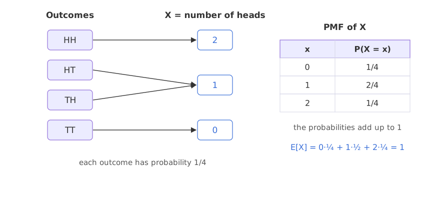
A capital letter (X) names the random variable and a small letter (x) one of its values, so P(X = 1) = 2/4 reads "the probability that the number of heads is 1".
Telling discrete and continuous random variables apart
- Discrete: the values can be counted, such as heads in 10 tosses, defective bulbs in a box or calls per hour. Bernoulli, binomial and Poisson variables are discrete.
- Continuous: any value in an interval is possible, such as a height, a waiting time or an income. Normal, log-normal and Pareto variables are continuous. The uniform distribution comes in both kinds.
Describing a discrete variable with a PMF
The probability mass function (PMF) gives the probability of each value: p(x) = P(X = x). Every p(x) lies between 0 and 1 and they add up to 1. For a fair die, p(x) = 1/6 for x = 1, 2, …, 6.
Describing a continuous variable with a PDF
A continuous variable has infinitely many values, so the chance of any one exact value is 0: P(X = 1.70000…) = 0 for a height. The probability density function (PDF) f(x) describes it instead, and probabilities are areas under it:
A density is not a probability. It can be larger than 1: a normal curve with standard deviation 0.1 has height 3.989 at its centre, while the area under it is still 1.
Accumulating probability with the CDF
The cumulative distribution function (CDF) works for both kinds: F(x) = P(X ≤ x). It climbs from 0 to 1. For a discrete variable it climbs in steps, one at each value; for a continuous one it climbs smoothly. A probability between two points is a difference of two CDF values: P(a < X ≤ b) = F(b) − F(a).
Finding the expected value and variance
The expected value E[X], also written μ, is the long-run average of X: each value weighted by its probability. The variance is the expected squared distance from μ, and the standard deviation is its square root.
For a fair die, E[X] = (1 + 2 + 3 + 4 + 5 + 6)/6 = 3.5, a value the die never shows: it is an average, not an outcome. The variance is 35/12 ≈ 2.9167. This is the population variance from Variance and standard deviation, with each value weighted by its probability instead of by 1/N.
Computing a distribution in Python
The code finds the die's mean and variance from its PMF with NumPy, checks them with scipy.stats.randint, compares them with 100,000 simulated rolls, and looks at a normal density.
import numpy as np
from scipy import stats

x = np.arange(1, 7)                      # the faces of a die
p = np.full(6, 1 / 6)                    # PMF: each face has probability 1/6
mean = np.sum(x * p)                     # E[X] = sum of x * p(x)
var = np.sum((x - mean) ** 2 * p)        # Var(X) = sum of (x - mean)^2 * p(x)
print("PMF adds up to", round(p.sum(), 10))
print("E[X] =", round(mean, 4), " Var(X) =", round(var, 4), " SD =", round(np.sqrt(var), 4))

die = stats.randint(1, 7)                # whole numbers 1 to 6: the upper end 7 is left out
print("scipy: mean", die.mean(), " var", round(die.var(), 4), " P(X <= 3) =", die.cdf(3))

rng = np.random.default_rng(42)
rolls = rng.integers(1, 7, size=100_000)
print("100,000 rolls: mean", round(rolls.mean(), 4), " variance", round(rolls.var(), 4))

z = stats.norm(0, 1)                     # a continuous variable
print("normal: pdf(0) =", round(z.pdf(0), 4), " P(X <= 0) =", z.cdf(0), " P(-1 < X <= 1) =", round(z.cdf(1) - z.cdf(-1), 4))
print("normal with sd 0.1: pdf(0) =", round(stats.norm(0, 0.1).pdf(0), 4))PMF adds up to 1.0 E[X] = 3.5 Var(X) = 2.9167 SD = 1.7078 scipy: mean 3.5 var 2.9167 P(X <= 3) = 0.5 100,000 rolls: mean 3.4998 variance 2.9173 normal: pdf(0) = 0.3989 P(X <= 0) = 0.5 P(-1 < X <= 1) = 0.6827 normal with sd 0.1: pdf(0) = 3.9894
Plotting a PMF, a PDF and their CDFs
import numpy as np
import matplotlib.pyplot as plt
from scipy import stats

fig, ax = plt.subplots(2, 2, figsize=(9, 6))
x = np.arange(1, 7)
ax[0, 0].bar(x, stats.randint(1, 7).pmf(x), width=0.4)
ax[0, 0].set_title("Fair die: PMF, P(X = x)")
xs = np.linspace(0, 7, 701)
ax[0, 1].plot(xs, stats.randint(1, 7).cdf(xs))
ax[0, 1].set_title("Fair die: CDF, steps of 1/6")
t = np.linspace(-4, 4, 400)
ax[1, 0].plot(t, stats.norm.pdf(t))
ax[1, 0].fill_between(t, stats.norm.pdf(t), where=(t > -1) & (t <= 1), alpha=0.3)
ax[1, 0].set_title("Standard normal: PDF, area = probability")
ax[1, 1].plot(t, stats.norm.cdf(t))
ax[1, 1].set_title("Standard normal: CDF, a smooth climb")
for a_ in ax.flat:
    a_.set_ylim(bottom=0)
fig.tight_layout()
plt.show()
print("die CDF at 3.5:", stats.randint(1, 7).cdf(3.5), " shaded normal area:", round(stats.norm.cdf(1) - stats.norm.cdf(-1), 4))die CDF at 3.5: 0.5 shaded normal area: 0.6827
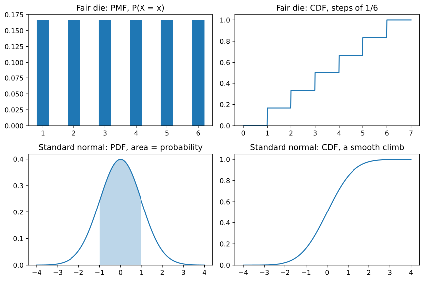
What the die and the normal curve show
- The PMF adds up to 1, as every PMF must.
- E[X] = 3.5, Var(X) = 2.9167 and SD = 1.7078, and scipy's
randint(1, 7)gives the same 3.5 and 2.9167. - P(X ≤ 3) = 0.5: the die's CDF at 3 adds the first three steps of 1/6.
- The simulated rolls land close: a mean of 3.4998 and a variance of 2.9173 from 100,000 rolls.
- The normal density at 0 is 0.3989, and the area between −1 and 1 is 0.6827, the 68% of the empirical rule. With a standard deviation of 0.1 the density at 0 is 3.9894, above 1, and it is still a valid density.
PMF vs PDF vs CDF
| PMF | CDF | ||
|---|---|---|---|
| For | Discrete variables | Continuous variables | Both |
| Gives | P(X = x) | A density f(x); areas are probabilities | P(X ≤ x) |
| Can exceed 1? | No | Yes | No |
| Die example | 1/6 for each face | None | 0.5 at x = 3 |
| scipy method | .pmf(x) | .pdf(x) | .cdf(x) |
Where you use random variables and distributions
- Modelling data: picking a distribution for counts, times or sizes tells you which tests and models fit.
- Expected values in decisions: the average payout of a bet, the expected number of returns from 1,000 orders.
- Simulation: drawing random values from a distribution to test a process before it runs for real.
Related
- Previous: Permutations and combinations
- Next: Bernoulli distribution
- Load a die that shows 6 half the time:
p = np.array([0.1] * 5 + [0.5]). What happens to E[X] and Var(X)? - Compute P(2 < X ≤ 5) for the fair die as
die.cdf(5) - die.cdf(2). Is it 3/6? - Find the area of the standard normal between −2 and 2 with
z.cdf(2) - z.cdf(-2).
Little by little, you're building something great.