
Probability basics
Probability is a number between 0 and 1 that measures how likely an event is: 0 means the event cannot happen and 1 means it is certain.
Last updated: 07 Oct, 2026 · SciPy 1.18
Normal (Gaussian) distribution and the lessons after it read probabilities as areas under a curve. Those areas rest on a few rules about chance, and every confidence interval and hypothesis test later on asks how likely a result would be by chance. Machine learning uses them too: a classifier such as Logistic regression returns the probability that a point belongs to class A or class B.
Defining probability with a die and a coin
The video defines probability as a measure of the likelihood of an event. Three words make that precise:
- Experiment: an action whose result is uncertain, such as rolling a die.
- Sample space: the set of every possible outcome. For a die it is {1, 2, 3, 4, 5, 6}; for a coin it is {H, T}.
- Event: a set of outcomes you care about. "Getting a 6" is the event {6}; "getting an even number" is {2, 4, 6}.
When every outcome is equally likely, the probability of an event is a count:
Rolling a 6 can happen in one way out of six outcomes, so P(6) = 1/6. A coin has two outcomes and heads is one of them, so P(H) = 1/2. An even number on a die can happen in three ways, so P(even) = 3/6 = 1/2.
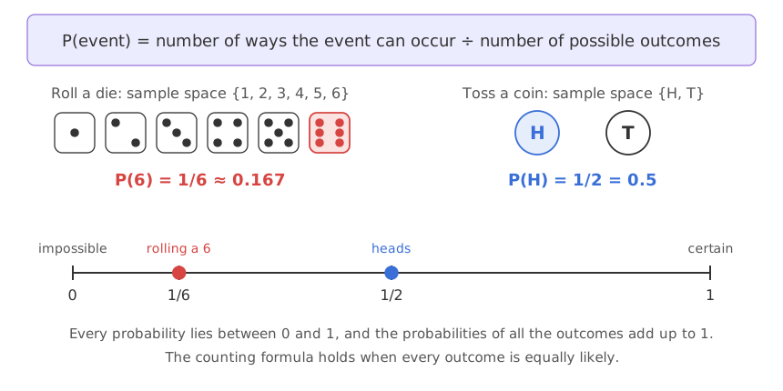
This counting rule is the classical definition. It holds only when the outcomes are equally likely, as with a fair die or a fair coin. A loaded die still has six outcomes, but they are not equally likely, so counting faces no longer gives the probability.
Reading probability as a long-run frequency
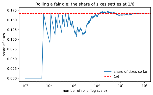
A second way to read a probability is as the share of times an event happens when the experiment is repeated many times. Roll a fair die 100,000 times and close to one roll in six is a 6. This relative frequency view is how a loaded die gets its probabilities: you roll it many times and count.
Whichever way a probability is found, it obeys three rules:
- It lies between 0 and 1: 0 ≤ P(A) ≤ 1 for every event A.
- The sample space is certain: P(S) = 1, so the probabilities of all the outcomes add up to 1 (six faces at 1/6 each make 1).
- Probabilities of events that cannot happen together add up: this is the addition rule, the topic of the next lesson.
Spotting mutually exclusive events
Two events are mutually exclusive when they cannot occur at the same time. On one roll of a die you get a 1 or a 2, never both. On one toss of a coin you get heads or tails, never both. For mutually exclusive events A and B, P(A and B) = 0. The addition rule lesson builds on this idea.
Using the complement rule
The complement of an event A, written "not A", is every outcome that is not in A. An event and its complement cover the sample space and cannot happen together, so their probabilities add up to 1:
The chance of not rolling a 6 is 1 − 1/6 = 5/6. The rule is most useful for "at least one" questions. The chance of at least one 6 in four rolls is 1 minus the chance of no 6 in all four rolls, which is (5/6)⁴ because the rolls do not affect each other (the multiplication rule lesson explains the product). So P(at least one 6) = 1 − (5/6)⁴ = 0.5177.
Computing probabilities by counting and by simulation
The code below counts outcomes with Fraction for exact answers, then rolls a simulated die 100,000 times with NumPy and watches the share of sixes.
from fractions import Fraction
import numpy as np

# classical probability: favourable outcomes / possible outcomes
die = [1, 2, 3, 4, 5, 6]
coin = ["H", "T"]
print("P(6) =", Fraction(sum(1 for x in die if x == 6), len(die)))
print("P(H) =", Fraction(coin.count("H"), len(coin)))
print("P(even) =", Fraction(sum(1 for x in die if x % 2 == 0), len(die)))

# long-run relative frequency of a 6
rng = np.random.default_rng(42)
rolls = rng.integers(1, 7, size=100_000)       # integers 1 to 6
for n in (10, 100, 1_000, 100_000):
    print(f"after {n:>6} rolls: share of sixes = {np.mean(rolls[:n] == 6):.4f}")
print("1/6 =", round(1 / 6, 4))

# complement rule: at least one six in four rolls
print("P(at least one 6 in 4 rolls) =", round(1 - (5 / 6) ** 4, 4))P(6) = 1/6 P(H) = 1/2 P(even) = 1/2 after 10 rolls: share of sixes = 0.1000 after 100 rolls: share of sixes = 0.1400 after 1000 rolls: share of sixes = 0.1590 after 100000 rolls: share of sixes = 0.1659 1/6 = 0.1667 P(at least one 6 in 4 rolls) = 0.5177
Plotting the share of sixes as the rolls add up
import numpy as np
import matplotlib.pyplot as plt

rng = np.random.default_rng(42)
rolls = rng.integers(1, 7, size=100_000)
n = np.arange(1, len(rolls) + 1)
share = np.cumsum(rolls == 6) / n              # share of sixes after each roll

plt.figure(figsize=(7, 4))
plt.plot(n, share, label="share of sixes so far")
plt.axhline(1 / 6, color="red", linestyle="--", label="1/6")
plt.xscale("log")
plt.title("Rolling a fair die: the share of sixes settles at 1/6")
plt.xlabel("number of rolls (log scale)")
plt.ylabel("share of sixes")
plt.legend()
plt.show()
print("share after 100,000 rolls:", round(share[-1], 4))share after 100,000 rolls: 0.1659
What the counts and the simulation show
- P(6) = 1/6, P(H) = 1/2 and P(even) = 1/2: the counts from the video's die and coin, kept as exact fractions.
- The share of sixes wanders early: 0.1000 after 10 rolls and 0.1400 after 100. A few rolls tell you little.
- It closes in on 1/6 later: 0.1590 after 1,000 rolls and 0.1659 after 100,000, against 1/6 = 0.1667. This is the long-run frequency reading of probability.
- At least one 6 in four rolls is 0.5177: a little better than even, found with the complement rule instead of listing all 1,296 sequences of four rolls.
Classical vs relative-frequency probability
| Classical | Relative frequency | |
|---|---|---|
| How it is found | Count favourable outcomes ÷ possible outcomes | Repeat the experiment, count how often the event happens |
| Needs | Equally likely outcomes | Many repetitions |
| Die example | P(6) = 1/6 exactly | 0.1659 after 100,000 rolls |
| Works for a loaded die | No | Yes |
Where you use probability
- Classification: a model reports P(spam) = 0.92 for an email instead of a bare label, and you choose the cut-off.
- Hypothesis tests: a p-value is a probability computed as if the null hypothesis were true.
- Risk and planning: the chance a delivery is late, a server fails or a patient responds to a drug.
Related
- Change the event to "a number greater than 4" with
x > 4. Do you get 1/3? - Change the seed to
default_rng(7). Do the early shares change much more than the share after 100,000 rolls? - Work out P(at least one 6 in 10 rolls) with the complement rule:
1 - (5/6) ** 10.
Little by little, you're building something great.