
Z-score and the standard normal distribution
A z-score is a standardized value that says how many standard deviations a value lies from the mean, z = (x − μ) / σ: positive above the mean, negative below it.
Last updated: 07 Oct, 2026 · SciPy 1.18
Empirical rule (68-95-99.7) talks in whole standard deviations. Most values fall between those steps, and the z-score says exactly where.
Measuring a value in standard deviations
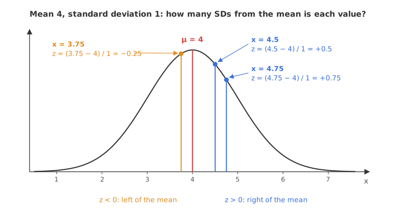
The video's dataset has mean 4 and standard deviation 1, so the axis runs 3, 2, 1 to the left of the mean and 5, 6, 7 to the right. Where does 4.5 fall? 5 is one standard deviation to the right, so 4.5 is half of one: +0.5 standard deviations.
For 4.75 the steps are harder to count by eye, so the video uses the z-score: the distance from the mean divided by the standard deviation.
For 4.75, z = (4.75 − 4)/1 = 0.75: 4.75 lies 0.75 standard deviations to the right of the mean. The sign gives the side; positive means right. For 3.75, z = (3.75 − 4)/1 = −0.25: a quarter of a standard deviation to the left.
A z-score has no units. Whether x is in runs, rupees or kilograms, the units cancel in (x − μ)/σ, which is what lets you compare values from different scales.
With data instead of a known population, use the sample mean x̄ and standard deviation s: z = (x − x̄)/s. Tools differ in which s they use. scipy.stats.zscore divides by n by default (ddof=0), the population formula from Variance and standard deviation.
Converting a normal distribution to the standard normal
Apply the z-score to every point on the axis of the video's N(4, 1): 1 becomes (1 − 4)/1 = −3, 2 becomes −2, 3 becomes −1, 4 becomes 0, and 5, 6, 7 become 1, 2, 3. The curve stays the same; only the axis is relabelled. The result is the standard normal distribution, the normal distribution with mean 0 and standard deviation 1, written Z ~ N(0, 1).
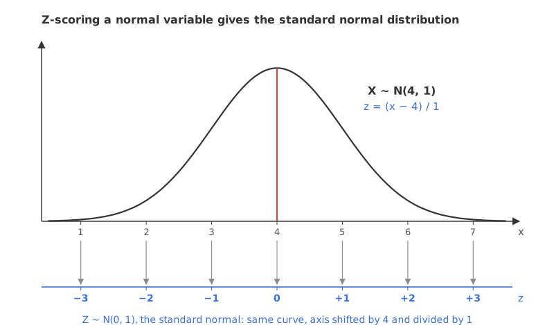
Every normal distribution turns into this one curve, so one table of Φ answers questions about all of them. That table is the subject of Z-table and normal probabilities.
Z-scoring a dataset keeps its shape
Z-scoring data, rather than the axis of a known distribution, uses the data's own mean and standard deviation. The seven values 1, 2, 3, 4, 5, 6 and 7 have mean 4 and a population standard deviation of 2, so their z-scores are (x − 4)/2: −1.5, −1, −0.5, 0, 0.5, 1 and 1.5.
Z-scored values always have mean 0 and standard deviation 1. Their shape does not change: z = (x − μ)/σ only shifts and rescales, so evenly spaced values stay evenly spaced, and skewed data stays skewed by the same amount. Z-scored data follows the standard normal distribution only when the original data was normal.
Computing z-scores in Python
One value by hand
mu, sigma = 4, 1
z = (4.75 - mu) / sigma        # 0.75: three quarters of an SD above the mean
A whole array with scipy.stats.zscore
import numpy as np
from scipy.stats import zscore

x = np.arange(1, 8)            # 1, 2, ..., 7
zscore(x) # (x - x.mean()) / x.std(), ddof=0 by defaultfrom scipy.stats import skew
for value in [4.5, 4.75, 3.75]:
print(f"x = {value}: z = {(value - 4) / 1:+.2f}") # mean 4, SD 1
print("mean and SD of 1..7:", x.mean(), x.std())
print("z-scores:", zscore(x))
print("mean and SD after:", zscore(x).mean(), zscore(x).std())
data = np.array([1, 2, 2, 3, 4, 5]) # a right-skewed set
print("skewness before:", round(skew(data), 4), " after:", round(skew(zscore(data)), 4))x = 4.5: z = +0.50 x = 4.75: z = +0.75 x = 3.75: z = -0.25 mean and SD of 1..7: 4.0 2.0 z-scores: [-1.5 -1. -0.5 0. 0.5 1. 1.5] mean and SD after: 0.0 1.0 skewness before: 0.3053 after: 0.3053
What the z-scores show
- 4.5, 4.75 and 3.75 give +0.50, +0.75 and −0.25, the distances the video reads off the curve.
- The values 1 to 7 have mean 4.0 and SD 2.0, so
zscorereturns −1.5 to 1.5 in steps of 0.5. - After z-scoring, the mean is 0.0 and the SD is 1.0, whatever the data.
- The skewness of 1, 2, 2, 3, 4, 5 is 0.3053 before and after: z-scoring moved and squeezed the data but kept its lopsided shape.
Population z-score vs sample z-score
| Population | Sample | |
|---|---|---|
| Formula | z = (x − μ)/σ | z = (x − x̄)/s |
| Centre and spread | Known parameters μ and σ | Estimated from the data |
| In scipy | norm(loc=μ, scale=σ) for curve questions | zscore(x) with ddof=0, or zscore(x, ddof=1) |
| Typical question | What share of IQs lie below 85 when μ = 100, σ = 15? | Which rows of this column are far from the rest? |
Where you use z-scores
- Comparing across scales. Two scores from different series or exams become comparable once each is measured in standard deviations of its own group; Z-table and normal probabilities does this for two cricket series.
- Outliers. |z| > 3 flags a value, as in Outlier detection with IQR and z-score.
- Feature scaling. Machine learning standardizes whole columns this way, in Standardization and normalization.
- Test statistics. The One-sample z-test applies the same idea to a sample mean.
Related
- Previous: Empirical rule (68-95-99.7)
- Next: Standardization and normalization
- See also: Variance and standard deviation
- Reference: scipy.stats.zscore
- Compute the z-score of 6.5 with mean 4: it is 2.5 when the SD is 1, and 1.25 when the SD is 2.
- Run
zscore(x, ddof=1): the values shrink a little, to −1.3887 for 1, because the sample SD of 1 to 7 is 2.1602. - Square
databefore z-scoring (data ** 2) and print the skewness: squaring changes the shape, z-scoring does not.
You understood something today that you didn't yesterday.